In this series, we attempt to understand GANs from the perspective of energy. We will find that this perspective is so beautiful and intuitive that it is truly impressive.
This perspective is directly inspired by the recent work from Yoshua Bengio’s team, “Maximum Entropy Generators for Energy-Based Models”, which appeared on arXiv a few days ago. Of course, the connection between energy-based models and GANs has a long history and is not an original invention of that paper; however, that paper executes the idea with more detail and refinement. Additionally, this article supplements those ideas with my own understanding and reflections, striving to be more accessible and complete.
As the first article in the series, we will start with a straightforward analogical derivation: GAN is essentially a journey of “digging holes” and “jumping into holes” (one after another)!
In general, the main contents of this article are as follows:
Providing a clear and intuitive energy visualization of GAN/WGAN;
Discussing the training conditions and strategies for the discriminator (energy function);
Pointing out a very beautiful and intuitive energy explanation for gradient penalty;
Discussing the choice of optimizers in GANs.
“Digging” and “Jumping”
In this section, we use a simple metaphor to explain what a GAN is from an energy perspective.
First, we have a set of samples x_1, x_2, \dots, x_n. We hope to find a generative model capable of creating a set of new samples \hat{x}_1, \hat{x}_2, \dots, \hat{x}_n, and we want these new samples to be very similar to the original ones. How do we create them? It’s simple; it involves two steps.
“Digging Holes”
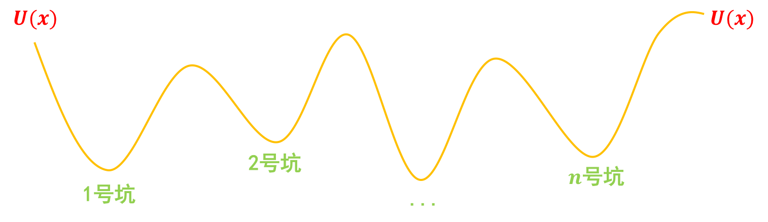
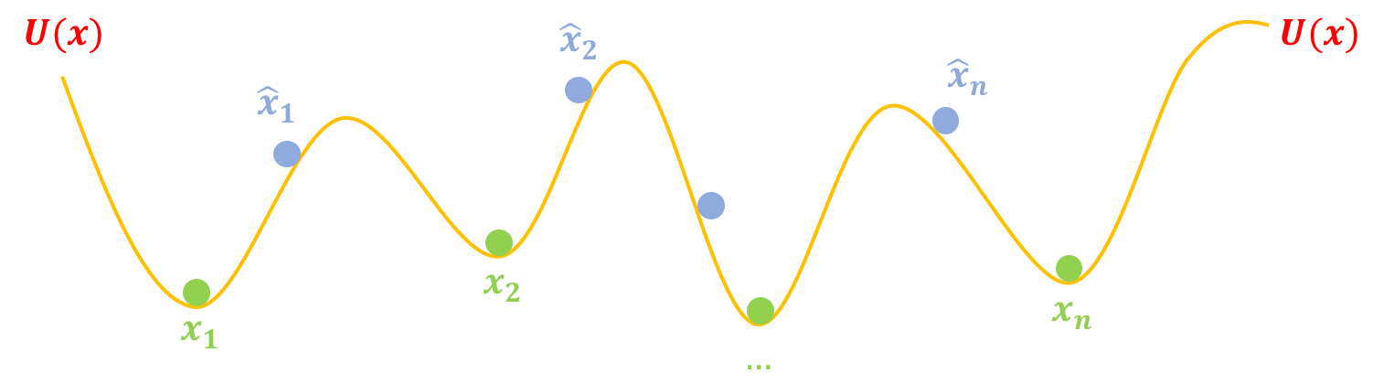
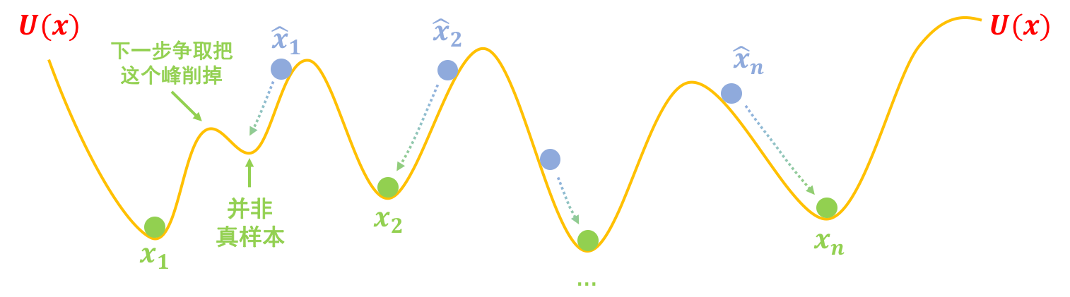
Step one: Digging holes. We treat the real samples x_1, x_2, \dots, x_n as coordinates and dig many holes at these locations. The distribution of these holes can be described by an energy function U(x). Consequently, the real samples x_1, x_2, \dots, x_n are all placed at the bottom of the holes. Then, we place the generated fake samples \hat{x}_1, \hat{x}_2, \dots, \hat{x}_n on the “slopes” of the holes:
“Jumping into Holes”
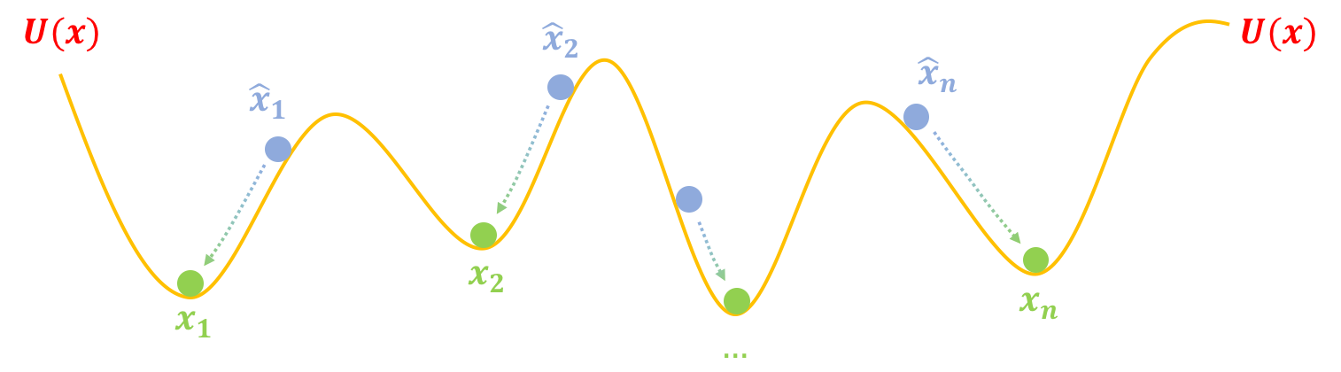
Step two: Jumping into holes. We fix U(x) (i.e., stop moving the holes) and then release the fake samples \hat{x}_1, \hat{x}_2, \dots, \hat{x}_n. Obviously, they will slowly roll down to the bottom of the holes. Since the bottom of the holes represents the real samples, \hat{x}_1, \hat{x}_2, \dots, \hat{x}_n all become very similar to the real samples:
This is the workflow of a GAN!
Formulating the GAN
Note that the two steps above are not just simple metaphors; they are a complete description of a GAN. Based on these two steps, we can directly write down the GAN training formulas.
The Discriminator
First, let’s look at “digging holes.” We said we want to put real samples at the bottom and fake samples on the slopes so that the fake samples can later roll to the bottom. This means the “average elevation” of the fake samples should be higher than the “average elevation” of the real samples. That is to say, we want: \mathbb{E}_{x\sim p(x)}\big[U(x)\big] - \mathbb{E}_{x\sim q(x)}\big[U(x)\big] \label{eq:eq-e} to be as small as possible. Here, we use p(x) to represent the distribution of real samples and q(x) to represent the distribution of fake samples. Fake samples are generated via x=G(z), where z\sim q(z) follows a standard normal distribution.
Gradient Penalty
Furthermore, we said real samples should be at the bottom of the holes. In mathematical terms, the bottom of a hole is a local minimum, where it is best if the derivative is zero, i.e., \nabla_x U(x)=0. In terms of an optimization objective, we want \Vert \nabla_x U(x)\Vert^2 to be as small as possible. Combining these, we get the optimization objective for U: \begin{aligned} U =& \mathop{\text{argmin}}_{U}\mathbb{E}_{x\sim p(x)}\big[U(x)\big] - \mathbb{E}_{x\sim q(x)}\big[U(x)\big] + \lambda \mathbb{E}_{x\sim p(x)}\big[\Vert \nabla_x U(x)\Vert^2\big]\\ =& \mathop{\text{argmin}}_{U}\mathbb{E}_{x\sim p(x)}\big[U(x)\big] - \mathbb{E}_{z\sim q(z)}\big[U(G(z))\big] + \lambda \mathbb{E}_{x\sim p(x)}\big[\Vert \nabla_x U(x)\Vert^2\big] \end{aligned} \label{eq:eq-ee}
Note: Previously, regarding gradient penalty, we always had two points of confusion: 1. Is it better for the gradient penalty to be centered at 0 or 1? 2. Should the gradient penalty be applied to real samples, fake samples, or interpolated samples? Now, based on the energy perspective, we can conclude that “applying a 0-centered gradient penalty to real samples” is better, because it means (globally) placing real samples at local minima.
Thus, from the energy perspective, we have a very intuitive answer for the gradient penalty.
The Generator
Next, let’s look at “jumping into holes.” Once the holes are dug and U is fixed, we let the fake samples roll to the bottom. This means decreasing U(x) so they roll into the nearest hole. Therefore: G = \mathop{\text{argmin}}_{G}\mathbb{E}_{z\sim q(z)}\big[U(G(z))\big] \label{eq:eq-g}
As we can see, the discriminator is essentially “creating a potential field,” and the generator is minimizing that potential energy. This is the main idea of the Energy GAN.
Alternating Training
If the distribution of holes in reality were as simple as the diagrams above, we might only need two steps to train a generative model. However, in reality, the distribution of holes can be very complex. For example, as shown in the figure below, as the fake sample \hat{x}_1 slowly slides down, it might not necessarily reach the hole of x_1, but rather an intermediate hole. This intermediate hole might not represent a real sample, but perhaps only a “semi-real” sample. Therefore, we need to continuously improve the fake samples and constantly correct the holes (for example, aiming to “shave off” the peaks blocking the path in the next step). This means we need to execute steps [eq:eq-e] and [eq:eq-g] repeatedly and alternately.
The Science of Holes
By simply imagining a few holes in our minds, we can derive the complete framework of a GAN, and it turns out to be an upgraded version of WGAN-GP: gradient penalty centered at 0.
A GAN is nothing more than the science of holes!
For further discussion on this GAN, you can refer to my previous blog post “WGAN-div: An Obscure WGAN Hole-Filler” or the paper “Which Training Methods for GANs do actually Converge?”.
Further Reflections
The aforementioned visualization can also help us answer many questions. For example, can the discriminator do without gradient penalty? Why is it that in GAN training—especially for the generator—most people do not use optimizers with momentum, or even if they do, they set the momentum very low? And how does mode collapse occur?
Hinge Loss
Gradient penalty is theoretically beautiful, but it is indeed too slow. From a practical standpoint, it is best to avoid it if possible. However, if we omit the gradient penalty and directly minimize Equation [eq:eq-e], numerical instability easily occurs.
This is not hard to understand. Without constraints, it is easy for U(x) \to -\infty for real samples and U(x) \to +\infty for fake samples. In other words, the discriminator is optimized too aggressively, and the gap becomes too large (infinite). A natural idea is to set a threshold for real and fake samples respectively, such that optimization stops once U(x) exceeds this threshold. For example: \mathbb{E}_{x\sim p(x)}\big[\max(0, 1+U(x))\big] + \mathbb{E}_{x\sim q(x)}\big[\max(0,1-U(x))\big] \label{eq:eq-e-hinge} In this way, for x\sim p(x), if U(x) < -1, then \max(0, 1+U(x))=0. For x\sim q(x), if U(x) > 1, then \max(0, 1-U(x))=0. In both cases, U(x) will no longer be optimized. This means U(x) doesn’t need to be too small for real samples and doesn’t need to be too large for fake samples, thereby preventing over-optimization of U(x).
This scheme is the Hinge Loss used by SNGAN, SAGAN, and BigGAN.
Of course, if U(x) itself is non-negative [for example, using the MSE of an autoencoder as U(x) in EBGAN], then Equation [eq:eq-e-hinge] can be slightly modified: \mathbb{E}_{x\sim p(x)}\big[U(x)\big] + \mathbb{E}_{x\sim q(x)}\big[\max(0,m-U(x))\big] \label{eq:eq-e-hinge2} where m > 0.
Optimizers
As for the choice of optimizer, the answer can be seen from the “jumping into holes” diagram.
Optimizers with momentum help us find better local minima faster. However, for GANs, we don’t actually need to reach a “better” (deeper) local minimum; we only need to reach the nearest local minimum. If we jump out of the nearest local minimum and run into a lower one, we might lose diversity or even encounter mode collapse.
For example, consider \hat{x}_2 in the figure below. An optimization algorithm without momentum allows \hat{x}_2 to stop at x_2. If momentum is used, it might overshoot x_2 and even end up at x_1. Although x_1 is also a real sample, this results in both \hat{x}_1 and \hat{x}_2 converging toward x_1. Consequently, there may be no fake samples left to generate x_2, leading to a loss of diversity.

Therefore, in GAN optimizers, the momentum should not be too large. If it is too large, it may lead to a loss of diversity in generated samples or cause other instabilities. Similarly, the learning rate should not be too large. In short, all acceleration methods should not be too aggressive.
Mode Collapse
What is mode collapse? Why does it happen? This can also be easily explained using this visualization.
Previously, we drew the fake samples \hat{x} in a reasonable way. However, if due to poor initialization or improper optimization, the \hat{x} samples cluster around only a few specific holes, for example:
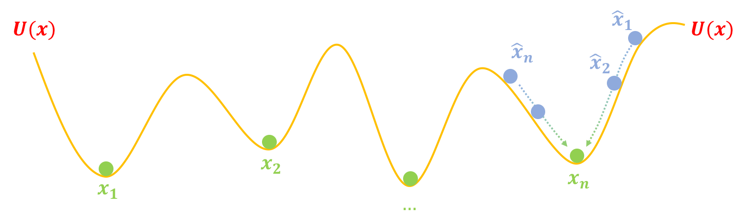
In this case, following the optimization process described above, all fake samples will rush toward x_n. Thus, the model can only generate a single (or a few) types of samples. This is mode collapse.
Simply put, mode collapse occurs because the fake samples are too concentrated and not “uniform” enough. Therefore, we can add a term to the generator to encourage the fake samples to be more uniform. This term is the entropy of the fake samples H(X)=H(G(Z)). We want the entropy of the fake samples to be as large as possible, which means they are more disordered and uniform. Thus, the generator’s objective can be changed to: G = \mathop{\text{argmin}}_{G} -H(G(Z)) + \mathbb{E}_{z\sim q(z)}\big[U(G(z))\big] \label{eq:eq-gg} Theoretically, this can solve the mode collapse problem. As for how to calculate H(X), we will discuss that in detail later.
The Beauty of the Energy Perspective
For GANs, the most popular perspective is the “forger vs. detective” competition analogy. This perspective directly led to the standard GAN. However, this popular analogy cannot be easily extended to understand WGAN or regularization terms like gradient penalty.
In contrast, the energy perspective is quite flexible. It even allows us to intuitively understand WGAN, gradient penalty, and other concepts, which are among the most advanced results in the GAN field today. Although the energy perspective seems formally more complex than the “forger-detective” model, its physical meaning is quite clear. With a little thought, one feels it is actually more interesting and enlightening—a concept that becomes more rewarding the more you chew on it.
Original address: https://kexue.fm/archives/6316
For more details on reprinting, please refer to: Scientific Space FAQ