WGAN-div: An Obscure Successor to WGAN

W-distance

WGAN introduces the Wasserstein distance from optimal transport to measure the distance between two distributions: W_c[\tilde{p}(x), q(x)] = \inf_{\gamma\in \Pi(\tilde{p}(x), q(x))} \mathbb{E}_{(x,y)\sim \gamma}[c(x,y)] Here, \tilde{p}(x) is the distribution of real samples, q(x) is the fake distribution, and c(x,y) is the transport cost. The paper uses c(x,y)=\Vert x-y\Vert. The notation \gamma\in \Pi(\tilde{p}(x), q(x)) means that \gamma is any joint distribution of x and y whose marginal distributions are \tilde{p}(x) and q(y). Intuitively, \gamma describes a transport plan, c(x,y) is the transport cost, and W_c[\tilde{p}(x), q(x)] represents the cost of the most efficient transport plan as the distance between distributions.

Dual Problem

The W-distance is indeed a good metric, but it is clearly difficult to calculate. When c(x,y)=\Vert x-y\Vert, we can transform it into its dual problem: W(\tilde{p}(x), q(x)) = \sup_{\Vert T\Vert_L\leq 1} \mathbb{E}_{x\sim \tilde{p}(x)}[T(x)] - \mathbb{E}_{x\sim q(x)}[T(x)] \label{eq:wgan-d} where T(x) is a scalar function and \Vert T\Vert_L is the Lipschitz norm: \Vert T\Vert_L = \max_{x\neq y} \frac{|T(x)-T(y)|}{\Vert x - y\Vert} In short, T(x) must satisfy: |T(x)-T(y)| \leq \Vert x - y\Vert

Generative Model

Consequently, the training of a generative model can be framed as a min-max problem under the W-distance: \mathop{\text{argmin}}_{G}\mathop{\text{argmax}}_{T,\Vert T\Vert_L\leq 1} \mathbb{E}_{x\sim \tilde{p}(x)}[T(x)] - \mathbb{E}_{x\sim q(z)}[T(G(z))] The first \text{argmax} attempts to obtain an approximate expression for the W-distance, while the second \text{argmin} attempts to minimize that distance.

However, T is not arbitrary; it must satisfy \Vert T\Vert_L\leq 1, known as the Lipschitz constraint (L-constraint). How should this constraint be applied? Thus, on one hand, WGAN pioneered a new school of GANs, raising GAN theory to a new height; on the other hand, WGAN also dug a massive pit regarding the L-constraint, which has led many researchers to jump in... (to fix it?)

Weight Clipping

This was the scheme proposed in the original WGAN paper: after each gradient descent step for the discriminator, the absolute values of the discriminator’s parameters are clipped to not exceed a fixed constant.

This is a very primitive approach and is basically no longer used. The idea is that the L-constraint essentially requires the network’s fluctuations not to exceed a linear function. Since activation functions usually satisfy this, one only needs to consider the network weights. The simplest solution is to directly limit the range of weights so that the network does not oscillate too violently.

Gradient Penalty

This approach is very direct: \Vert T\Vert_L\leq 1 can be guaranteed by \Vert \nabla T\Vert \leq 1. Therefore, the gradient of the discriminator is added as a penalty term to the discriminator’s loss: T=\mathop{\text{argmin}}_{T} -\mathbb{E}_{x\sim \tilde{p}(x)}[T(x)] + \mathbb{E}_{x\sim q(x)}[T(x)] + \lambda \mathbb{E}_{x\sim r(x)}\Big[\big(\Vert \nabla T\Vert - 1\big)^2\Big] But the problem is that we require \Vert T\Vert_L\leq 1 to hold everywhere, so r(x) should ideally be a uniform distribution over the entire space, which is obviously difficult to achieve. Thus, the authors adopted a very clever (and somewhat “rogue”) approach: penalizing random interpolations between real and fake samples, ensuring the transition region between them satisfies the L-constraint.

This scheme is WGAN-GP. Clearly, it is more sophisticated than weight clipping and usually works very well. However, it is a heuristic scheme without more complete theoretical support.

Spectral Normalization

Another scheme to implement the L-constraint is Spectral Normalization (SN). You can refer to my previous post “Lipschitz Constraints in Deep Learning: Generalization and Generative Models”.

Essentially, Spectral Normalization and weight clipping belong to the same category of solutions, but Spectral Normalization has a more complete theory and yields more relaxed results. Another difference is that weight clipping is an “after-the-fact” processing scheme (clipping parameters after each gradient descent), which can lead to optimization instability. Spectral Normalization is a “pre-emptive” scheme; it spectrally normalizes the weights of each layer before computation. As part of the model, it is more reasonable.

Despite being more sophisticated, Spectral Normalization shares a problem with weight clipping: it restricts the discriminator to a small family of functions. That is, T with Spectral Normalization is only a small subset of all functions satisfying the L-constraint. This is because Spectral Normalization effectively requires every layer of the network to satisfy the L-constraint. This condition is too rigid; perhaps one layer could violate the L-constraint while the next satisfies a stronger one, canceling each other out so the whole network satisfies the constraint. Spectral Normalization cannot adapt to such cases.

Paper Review

Is there such a good thing? Let’s see what W-divergence is. Right at the start, the authors review some classic GAN training schemes and then casually cite a paper titled “Partial differential equations and monge-kantorovich mass transfer”. This paper provides a scheme (the order of presentation here differs from the original paper) that can directly train T. The objective is: T^* = \mathop{\text{argmax}}_{T} \mathbb{E}_{x\sim \tilde{p}(x)}[T(x)] - \mathbb{E}_{x\sim q(x)}[T(x)] - \frac{1}{2}\mathbb{E}_{x\sim r(x)}[\Vert \nabla T\Vert^2] \label{eq:wgan-div-d1} Here r(x) is a very loose distribution, which we will discuss later. The meaning of the entire loss is: as long as you train T according to this formula, it will be the optimal solution for T in equation [eq:wgan-d]. Then, by substituting it into equation [eq:wgan-d], you obtain the W-distance. Minimizing this distance allows you to train the generator: \mathop{\text{argmin}}_{G}\mathbb{E}_{x\sim \tilde{p}(x)}[T^*(x)] - \mathbb{E}_{x\sim q(z)}[T^*(G(z))] \label{eq:wgan-div-g1}

Some Annotations

First, why did I say the authors “casually” cited a paper? Because they really did...

The authors simply state “According to [19]”, and then provide the results. [19] is that paper—a 59-page work on optimal transport and partial differential equations... I flipped through it and finally found that the authors were likely citing results from pages 36 and 40 (though I couldn’t understand them further and gave up). They didn’t provide much more reference material, which is a bit awkward. For some subsequent lemmas, the authors also say “refer to the discussion in [19]”...

Furthermore, readers might wonder: how is this different from the gradient penalty scheme? Isn’t adding a negative sign to minimize it basically the same? In experiments, there might not be much difference, but theoretically, the difference is significant. WGAN-GP’s gradient penalty is just a heuristic, while equation [eq:wgan-div-d1] has theoretical guarantees. We will continue to explain this.

W-divergence

Equation [eq:wgan-div-d1] is a theoretical result. Since deep learning is a combination of theory and engineering, the authors considered a more generalized objective: W_{k,p}[\tilde{p}(x), q(x)] = \max_{T} \mathbb{E}_{x\sim \tilde{p}(x)}[T(x)] - \mathbb{E}_{x\sim q(x)}[T(x)] - k\mathbb{E}_{x\sim r(x)}[\Vert \nabla T\Vert^p] \label{eq:wdiv} where k > 0, p > 1. Based on this, the authors proved that W_{k,p} has very good properties:

1. W_{k,p} is a symmetric divergence. A divergence means: \mathcal{D}[P,Q]\geq 0 and \mathcal{D}[P,Q]=0 \Leftrightarrow P=Q. The difference from a “distance” is that it doesn’t necessarily satisfy the triangle inequality; it is sometimes called a “semi-metric” or “quasi-distance.” The fact that W_{k,p} is a divergence is already excellent because most GANs are just optimizing some divergence. A divergence implies that when we minimize it, we are truly reducing the distance between two distributions.

2. The optimal solution of W_{k,p} is related to the W-distance. Equation [eq:wgan-div-d1] is a special case of W_{1/2,2}. This shows that after maximizing W_{k,p} to get T, we can remove the gradient term and train the generator by minimizing [eq:wgan-div-g1]. This also indicates that using W_{k,p} as an objective yields properties similar to the W-distance, avoiding vanishing gradient problems.

3. This is the most amusing point: the authors proved that \max_{T} \mathbb{E}_{x\sim \tilde{p}(x)}[T(x)] - \mathbb{E}_{x\sim q(x)}[T(x)] - k\mathbb{E}_{x\sim r(x)}[(\Vert \nabla T\Vert - n)^p] is not always a divergence. When n=1, p=2, this is the WGAN-GP gradient penalty. The authors state it is not a divergence, clearly taking a shot at WGAN-GP, haha! Not being a divergence means that when WGAN-GP trains the discriminator, it isn’t always increasing the distance between the two distributions (the discriminator is slacking off and not improving its skills), which leads to inaccurate gradients being backpropagated to the generator.

WGAN-div

Finally, we can introduce WGAN-div, which is the WGAN training mode based on equation [eq:wdiv]: \begin{aligned} T &= \mathop{\text{argmax}}_{T} \mathbb{E}_{x\sim \tilde{p}(x)}[T(x)] - \mathbb{E}_{x\sim q(x)}[T(x)] - k\mathbb{E}_{x\sim r(x)}[\Vert \nabla T\Vert^p] \\ G &= \mathop{\text{argmin}}_{G} \mathbb{E}_{x\sim \tilde{p}(x)}[T(x)] - \mathbb{E}_{x\sim q(z)}[T(G(z))] \end{aligned} The former uses W-divergence W_{k,p} to find the optimal T for the W-distance, and the latter minimizes the W-distance. Thus, the role of W-divergence is that of an obscure successor fixing the holes in WGAN. Combined with the fact that this paper itself has received little attention, this feeling is even stronger.

Choice of k, p

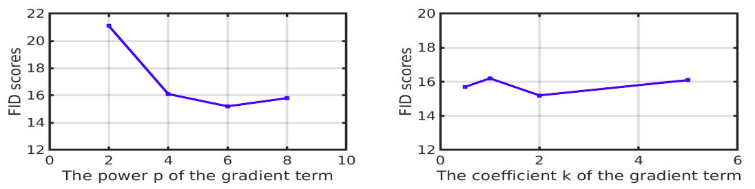
Through a series of search experiments, the authors found that k=2, p=6 yielded the best results (using FID as the metric). This further diverges from WGAN-GP: a quadratic power of the norm is not necessarily the best choice.

Choice of r(x)

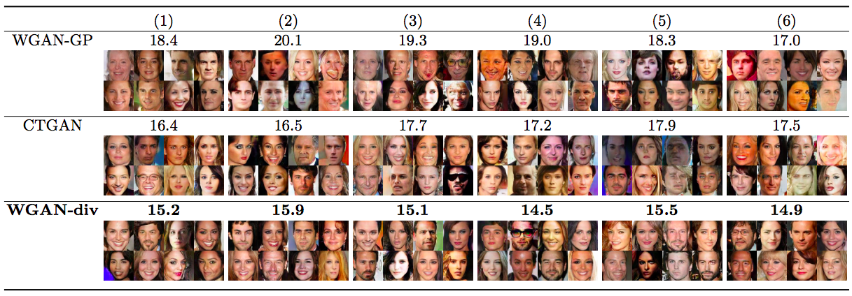
As mentioned earlier, the requirements for r(x) in W-divergence are very loose. The paper conducted a set of comparative experiments on common practices:

1. Random interpolation between real and fake samples;
2. Random interpolation between real samples, and between fake samples;
3. Mixing real and fake samples, then randomly selecting two for interpolation;
4. Directly mixing original real and fake samples;
5. Selecting only original fake samples;
6. Selecting only original real samples.

The results showed that under WGAN-div, these methods performed similarly (using FID). However, for WGAN-GP, the differences were significant, and the best result for WGAN-GP was worse than the worst result for WGAN-div. At this point, WGAN-GP was completely outperformed...

The difference is easy to explain: WGAN-GP adds a gradient penalty based on experience, and “random interpolation between real and fake samples” is just a compromise because it cannot sample the entire space. However, W-divergence and WGAN-div, from their theoretical inception, do not have strict restrictions on r(x). In fact, the construction of the original W-divergence (which requires looking at the reference paper) basically only requires r(x) to be a distribution over the same sample space as \tilde{p}(x) and q(x). This is a very weak requirement, and we generally choose a distribution derived from both \tilde{p}(x) and q(x) for relatively faster convergence.

Reference Code

Naturally, it’s written in Keras—Life is short, I use Keras:
https://github.com/bojone/gan/blob/master/keras/wgan_div_celeba.py

Random samples (my own experimental results):

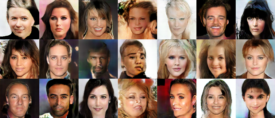
Of course, the experimental results in the original paper also show that WGAN-div is excellent: