Friends working in computer vision may know that AM-Softmax is a result from face recognition research. This article draws on face recognition practices to build a sentence similarity model and introduces how to write various margin losses in Keras.
Background
Upon closer reflection, one finds many similarities between sentence similarity and face recognition.
Existing Approaches
In the materials I have searched, there are generally only two ways to build sentence similarity models using deep learning. One is to input a pair of sentences and output a 0/1 label representing the degree of similarity, treating it as a binary classification problem. For example, the model in "Learning Text Similarity with Siamese Recurrent Networks" looks like this:

This includes competitions like Paipaidai’s "Mirror Cup" this year. Another approach is to input a triplet "(Sentence A, sentence similar to A, sentence dissimilar to A)" and solve it using triplet loss, as seen in the paper "Applying Deep Learning To Answer Selection: A Study And An Open Task".
These two approaches can actually be seen as one; they are essentially the same, with differences only in the loss function and training method. However, both methods suffer from a serious problem: severe undersampling of negative samples, leading to very slow performance improvement.
Usage Scenarios
Let’s review the scenarios where we use sentence similarity models. Generally, we have pre-stored many FAQ pairs, i.e., "Question-Answer" pairs. When we encounter a new question, we need to compare its similarity with all questions in the original database, find the most similar one, and decide whether to provide an answer based on the similarity and a threshold.
Note that this involves two elements. First is "all": theoretically, we compare the new question with every question in the database to find the most similar one. Second is the "threshold": we don’t know if the new question has an answer in the database, so this threshold determines whether we respond. If we simply take the top-1 result regardless of the score, the user experience will be poor.
We are mainly concerned with "all" (in fact, if "all" is solved, the "threshold" is also solved). "All" means that during training, for each sentence, except for the few similar sentences which are positive samples, all other sentences should serve as negative samples. But with the previous approaches, it is difficult to sample all negative samples completely, and even if possible, the training time would be extremely long. This is the drawback mentioned earlier.
Help from Face Recognition
I have always felt that in the field of machine learning, one should not "draw lines" too strictly. For example, some readers think they do NLP and thus don’t touch images, and vice versa. In fact, the gaps between different fields of machine learning are not that large; many things are essentially the same, just in different scenarios. For instance, the so-called sentence similarity model almost perfectly corresponds to the face recognition task, and face recognition is currently quite mature, so we can clearly learn from it.
Setting aside models for a moment, let’s imagine a face recognition scenario. For example, a company uses face recognition for clocking in. Once a face recognition model is available, we pre-store face photos of employees. Every day, we take a photo of an employee (real-time, obviously not perfectly matching the stored photo), and we need to determine if they are an employee and, if so, which one.
Imagine replacing "face" with "sentence" in the above scenario—isn’t that exactly the usage scenario for a sentence similarity model?
Clearly, the sentence similarity model can be considered the face recognition of NLP.
Model
Sentence similarity and face recognition are similar in all aspects: from model usage to construction and even the scale of datasets. Therefore, almost all models and techniques from face recognition can be applied to sentence similarity models.
As a Classification Problem
In fact, the triplet loss mentioned earlier is also one of the standard methods for training face recognition models. Triplet loss itself is not wrong; if parameters are fine-tuned and it is retrained, the effect can be very good. However, in many cases, it is simply too inefficient. Currently, a more standard approach is to treat it as a multi-class classification problem.
For example, suppose there are 100,000 different people in the training set, with 5 face images per person, totaling 500,000 training images. We then train a CNN model to extract features and build a 100,000-class classification model. Yes, it’s a classification problem just like MNIST, but with a much larger number of classes—as many classes as there are different people. Sentence similarity can be handled similarly: the training set can be divided into many groups of "synonymous sentences," and there are as many classes as there are groups.
Note that this is only for training; the final classification model might be useless. This is easy to imagine: we can use an existing face database to train a model, but our usage scenario might be company check-ins, meaning the faces to be recognized are those of internal employees who are clearly not in the public database. So the classification model is meaningless; what is truly meaningful is the feature extraction model before the classification layer. For example, a typical CNN classification model can be simplified into two steps: \begin{aligned} \boldsymbol{z} &= CNN(\boldsymbol{x}) \\ \boldsymbol{p} &= \text{softmax}(\boldsymbol{z}\boldsymbol{W}) \end{aligned} where \boldsymbol{x} is the input, \boldsymbol{p} is the probability output for each class, and the softmax here does not include a bias term. When training as a classification problem, we output the face image \boldsymbol{x} and the corresponding one-hot label \boldsymbol{p}. But during usage, we don’t use the whole model; we only use the CNN(\boldsymbol{x}) part, which is responsible for converting each face image into a fixed-length vector.
With this transformation model (encoder), we can encode new faces in any scenario and then compare these encoded vectors, thus removing dependence on the original classification model. Therefore, the classification model is a training scheme; once training is complete, it retires, leaving behind the encoding model.
Classification vs. Ranking
Is that enough? Not yet. As mentioned, what we truly want is a feature extraction model (encoder) and to use the classification model as a training scheme, while the final method of use is to compare and rank the features.
We want to do feature ranking, but we use a classification model for training. Are these two equivalent?
The answer is: related but not equivalent. How does a classification problem work? Intuitively, it selects some class centers and says:
Each sample belongs to the class of the center closest to it.
Of course, these class centers are also trained, and the "distance" here can have various possibilities, such as Euclidean distance, cosine value, or inner product. Standard softmax corresponds to the inner product. This approach to classification leads to the following possible results:
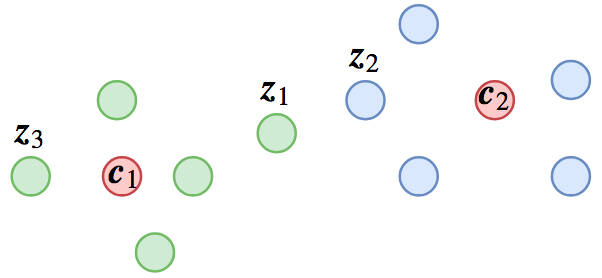
What is the problem with this classification result? Look at the three samples \boldsymbol{z}_1, \boldsymbol{z}_2, \boldsymbol{z}_3 in the figure. \boldsymbol{z}_1 and \boldsymbol{z}_3 are closest to \boldsymbol{c}_1, so they belong to Class 1. \boldsymbol{z}_2 is closest to \boldsymbol{c}_2, so it belongs to Class 2. Assuming this classification is correct, \boldsymbol{z}_1 and \boldsymbol{z}_3 might be synonymous sentences, while \boldsymbol{z}_2 is not synonymous with them; or \boldsymbol{z}_1 and \boldsymbol{z}_3 are face images of the same person, while \boldsymbol{z}_2 is someone else.
From a classification perspective, this result is reasonable. But as we said, we don’t want the classification model; we need to compare features. The problem is obvious: \boldsymbol{z}_1 and \boldsymbol{z}_2 are very close but belong to different classes, while \boldsymbol{z}_1 and \boldsymbol{z}_3 are far apart but belong to the same class. If we use feature ranking to find a synonym for \boldsymbol{z}_1, we would find \boldsymbol{z}_2 instead of \boldsymbol{z}_3, leading to an error.
Loss
What was described above is the non-equivalence of classification and ranking. That is, classification is correct, but feature ranking is wrong. Of course, as seen from the figure, although not completely equivalent, the classification model still gives most features a reasonable distribution; problems only occur for features near the boundaries.
Margin Softmax
One can imagine that the problem occurs at points near the classification boundaries. The reason is that the classification condition is too loose. If we tighten the classification condition, we can improve the ranking effect. For example:
The distance between each sample and its own class center must be less than half of its distance to other class centers.
Originally, we only needed it to be less than the distance to other classes; now, we also need it to be less than half of that distance. Clearly, the condition is tightened. The classification result shown in the previous figure would no longer be good enough because although \|\boldsymbol{z}_1 - \boldsymbol{c}_1\| < \|\boldsymbol{z}_1 - \boldsymbol{c}_2\|, it does not satisfy \|\boldsymbol{z}_1 - \boldsymbol{c}_1\| < \frac{1}{2}\|\boldsymbol{z}_1 - \boldsymbol{c}_2\|. Thus, the loss needs further optimization.
If training is completed according to this condition, we can imagine that the distance between \boldsymbol{z}_1 and \boldsymbol{z}_2 is pushed apart, while the distance between \boldsymbol{z}_1 and \boldsymbol{z}_3 is reduced. This is exactly the result we hope for: increasing inter-class distance and decreasing intra-class distance.
In fact, the scheme described above is essentially the famous L-Softmax in face recognition. In the field of face recognition, many similar losses have been proposed, all designed to address the non-equivalence between classification and ranking, such as A-Softmax, AM-Softmax, and AAM-Softmax. They are collectively called Margin Softmax. Furthermore, there are not only Margin Softmax but also Center Loss, improved versions of Triplet Loss, and so on.
AM-Softmax
I am not an image processing expert, so I won’t continue the story of face recognition. Let’s return to the main topic. As mentioned, face recognition cannot use pure softmax classification; it must use Margin Softmax. Because of the similarity between sentence similarity and face recognition models, sentence similarity models also need Margin Softmax. In short, we should at least pick one Margin Softmax to implement.
Among them, the scheme with good results and the easiest implementation is AM-Softmax. This article uses it as an example to introduce this type of Margin Softmax implementation and ultimately build a sentence similarity model.
The approach of AM-Softmax is actually very simple. Originally, softmax is \boldsymbol{p}=\text{softmax}(\boldsymbol{z}\boldsymbol{W}). Let \boldsymbol{W} = (\boldsymbol{c}_1, \boldsymbol{c}_2, \dots, \boldsymbol{c}_n) Then softmax can be rewritten as \boldsymbol{p}=\text{softmax}(\langle\boldsymbol{z},\boldsymbol{c}_1\rangle, \langle\boldsymbol{z},\boldsymbol{c}_2\rangle, \dots, \langle\boldsymbol{z},\boldsymbol{c}_n\rangle) The loss is the cross-entropy: -\log p_t = - \log \frac{e^{\langle\boldsymbol{z},\boldsymbol{c}_t\rangle}}{\sum_{i=1}^n e^{\langle\boldsymbol{z},\boldsymbol{c}_i\rangle}} where t is the target label. AM-Softmax does two things:
Performs L2 normalization on both \boldsymbol{z} and \boldsymbol{c}_i, meaning the inner product becomes a cosine value.
Subtracts a positive number m from the target cosine value and then applies a scaling factor s.
The loss becomes: -\log p_t = - \log \frac{e^{s\cdot(\cos\theta_t -m)}}{e^{s\cdot (\cos\theta_t -m)}+\sum_{i\neq t} e^{s\cdot\cos\theta_i }} where \theta_i represents the angle between \boldsymbol{z} and \boldsymbol{c}_i. In the original AM-Softmax paper, s=30 and m=0.35 are used.
From AM-Softmax, we can see the solution to the previously mentioned problem. First, the existence of s is necessary because the range of cosine is [-1, 1]. Scaling is needed to allow p_t to be close enough to 1 (if necessary). Of course, s does not change the relative order, so it is not the core change. The core change is replacing \cos\theta_t with \cos\theta_t - m.
Margin at Will
As mentioned earlier, the non-equivalence between classification and feature ranking can be solved by strengthening the classification condition. "Strengthening" simply means using a new function \psi(\theta_t) to replace \cos\theta_t, as long as: \psi(\theta_t) < \cos\theta_t Any such function can be considered a strengthening. AM-Softmax takes \psi(\theta_t) = \cos\theta_t - m, which is likely the simplest and most direct scheme satisfying the above inequality (fortunately, it also works very well).
Understanding this idea, we can construct various \psi(\theta_t), as theoretically any function satisfying (6) can be chosen. We also mentioned L-Softmax and A-Softmax, which essentially choose \psi(\theta_t) = \cos m\theta_t, where m is an integer. However, we know that \cos m\theta_t < \cos \theta_t is not always true, so the papers constructed a piecewise function based on \cos m\theta_t, which is quite cumbersome and makes the model extremely difficult to converge. In fact, I have tested the following method: \psi(\theta_t) = \min(\cos m\theta_t, \cos\theta_t) The results are comparable to AM-Softmax (on the sentence similarity task). Thus, the above can serve as a simple alternative to L-Softmax and A-Softmax; I call it simpler-a-softmax. Interested readers can try its effect on faces.
Implementation
Finally, I will introduce the Keras implementation of these losses. The test environment is Python 2.7, Keras 2.1.5, with a TensorFlow backend.
Basic Implementation
Implementing AM-Softmax in the most basic way is not difficult:
from keras.models import Model
from keras.layers import *
import keras.backend as K
from keras.constraints import unit_norm

x_in = Input(shape=(maxlen,))
x_embedded = Embedding(len(chars)+2, word_size)(x_in)
x = CuDNNGRU(word_size)(x_embedded)
x = Lambda(lambda x: K.l2_normalize(x, 1))(x)

pred = Dense(num_train,
             use_bias=False,
             kernel_constraint=unit_norm())(x)

encoder = Model(x_in, x) # The goal is to get an encoder
model = Model(x_in, pred) # Use classification for training

def amsoftmax_loss(y_true, y_pred, scale=30, margin=0.35):
    y_pred = y_true * (y_pred - margin) + (1 - y_true) * y_pred
    y_pred *= scale
    return K.categorical_crossentropy(y_true, y_pred, from_logits=True)

model.compile(loss=amsoftmax_loss,
              optimizer='adam',
              metrics=['accuracy'])
Sparse Version Implementation
The code above is easy to understand, mainly relying on
y_true being a one-hot input. This allows using simple
multiplication to extract the target cosine value, subtract the margin,
and then add back the other parts.
If you are just playing with a 10-class problem like MNIST, the code
above is perfectly sufficient. But in face recognition or sentence
similarity scenarios, we are dealing with tens of thousands or even
hundreds of thousands of classes. In this case, using one-hot input is
very memory-intensive (and preparing the data is also more troublesome).
Ideally, we want y_true to just be the integer ID of the
corresponding class. For standard cross-entropy, Keras provides
sparse_categorical_crossentropy. Can we write a Sparse
version for AM-Softmax?
One simple way is to include the one-hot conversion inside the loss function:
def sparse_amsoftmax_loss(y_true, y_pred, scale=30, margin=0.35):
    y_true = K.cast(y_true[:, 0], 'int32') # Ensure y_true shape=(None,), dtype=int32
    y_true = K.one_hot(y_true, K.int_shape(y_pred)[-1]) # Convert to one-hot
    y_pred = y_true * (y_pred - margin) + (1 - y_true) * y_pred
    y_pred *= scale
    return K.categorical_crossentropy(y_true, y_pred, from_logits=True)
This does achieve the goal, but it merely shifts the problem and
doesn’t truly skip the one-hot conversion. We can use TensorFlow’s
gather_nd function to truly skip the one-hot conversion.
Here is the reference code:
def sparse_amsoftmax_loss(y_true, y_pred, scale=30, margin=0.35):
    y_true = K.expand_dims(y_true[:, 0], 1) # Ensure y_true shape=(None, 1)
    y_true = K.cast(y_true, 'int32') # Ensure y_true dtype=int32
    batch_idxs = K.arange(0, K.shape(y_true)[0])
    batch_idxs = K.expand_dims(batch_idxs, 1)
    idxs = K.concatenate([batch_idxs, y_true], 1)
    y_true_pred = K.tf.gather_nd(y_pred, idxs) # Extract target features using tf.gather_nd
    y_true_pred = K.expand_dims(y_true_pred, 1)
    y_true_pred_margin = y_true_pred - margin # Subtract margin
    _Z = K.concatenate([y_pred, y_true_pred_margin], 1) # To calculate partition function
    _Z = _Z * scale # Scale results, since pred is cosine in [-1, 1]
    logZ = K.logsumexp(_Z, 1, keepdims=True) # Use logsumexp to prevent gradient vanishing
    logZ = logZ + K.log(1 - K.exp(scale * y_true_pred - logZ)) # Subtract exp(scale * y_true_pred) from Z
    return - y_true_pred_margin * scale + logZ
This code is slightly faster than the one-hot version. The key is
using tf.gather_nd to extract the target column and then
using logsumexp to calculate the log-partition function,
which is likely the standard way to implement cross-entropy. Based on
this, other forms of margin softmax loss can be implemented. Now you can
input only class IDs, just like with
sparse_categorical_crossentropy. Other frameworks can
follow this implementation.
Results Preview
A complete sentence similarity model can be found here:
https://github.com/bojone/margin-softmax/blob/master/sent_sim.py
This is a character-based model using GRU as the encoder. The corpus
used is tongyiju.csv as shown (the corpus is not shared;
readers who want to run it should prepare their own corpus in the same
format):
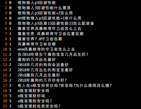
The ID at the beginning represents the sentence group, separated by
\t. Sentences in the same group are considered synonymous,
while sentences in different groups are non-synonymous.
Training Results: On the classification problem of
the training set, it can reach 90%+ accuracy. On the validation set
(evaluate function), the top-1, top-5, and top-10
accuracies for several losses are as follows (without fine-tuning):
| top1 acc | top5 acc | top10 acc | |
|---|---|---|---|
| softmax | 0.9077 | 0.9565 | 0.9673 |
| AM-Softmax | 0.9172 | 0.9607 | 0.9709 |
| simpler-asoftmax | 0.9135 | 0.9587 | 0.9697 |
It is worth mentioning that the
evaluate function is tested entirely according to the real
usage environment. That is, none of the sentences in the validation set
appeared in the training set. When running the evaluate
function, ranking is performed only within the validation set. If a
synonym of the input sentence appears in the top n sentences after ranking by similarity, the
top-n hit count increases by
1.
Therefore, the accuracy is quite impressive and meets engineering requirements. Below are a few randomly selected matching examples:
ll Source Sentence & Guangzhou’s
passenger station count
Similarity Ranking &
| Similar Sentence | Similarity |
|---|---|
| How many passenger stations are in Guangzhou? | 0.8281 |
| How many bus passenger stations are in Guangzhou? | 0.7980 |
| How many passenger stations are in Tianhe, Guangzhou? | 0.6781 |
| How many bus passenger stations are in Tianhe District, Guangzhou? | 0.6527 |
ll Source Sentence & How high is a
sofa generally
Similarity Ranking &
| Similar Sentence | Similarity |
|---|---|
| What is the general height of a sofa? | 0.8658 |
| How high is a living room sofa generally? | 0.7458 |
| What is the ordinary height of a general sofa? | 0.7173 |
| What are the general height dimensions of a sofa? | 0.6872 |
ll Source Sentence & Can PS format
be converted to AI format
Similarity Ranking &
| Similar Sentence | Similarity |
|---|---|
| How to convert a PS format image to an AI format image? | 0.9351 |
| What format should a Photoshop file be saved in to open in AI? | 0.6825 |
| PS files can be changed to AI format files | 0.6531 |
| Conversion mode for video format conversion | 0.5880 |
Conclusion
This article explains my understanding of sentence similarity models. I believe the best approach is not binary classification or triplet loss, but rather imitating the margin loss used in face recognition. This is the fastest way to improve performance. Of course, I haven’t exhaustively compared all methods; I simply felt it should be that way based on my superficial understanding of face recognition. Readers are welcome to test and discuss this further.
Original address: https://kexue.fm/archives/5743
For more details on reprinting, please refer to: "Scientific Space FAQ"