A Unified Understanding of Generative Models via Variational Inference (VAE, GAN, AAE, ALI)

VAE

In VAE, we set q(x,z)=q(x|z)q(z) and p(x,z)=\tilde{p}(x) p(z|x), where q(x|z) and p(z|x) are Gaussian distributions with unknown parameters, and q(z) is a standard Gaussian distribution. The objective to minimize is: \label{eq:kl-oo} KL\left(p(x,z)\Vert q(x,z) \right)=\iint \tilde{p}(x) p(z|x) \log \frac{\tilde{p}(x) p(z|x)}{q(x|z)q(z)}dxdz Since \log \tilde{p}(x) does not contain optimization parameters, it can be regarded as a constant, and the integral over \tilde{p}(x) is transformed into sampling from the data, thus: \mathbb{E}_{x\sim \tilde{p}(x)}\left[-\int p(z|x)\log q(x|z)dz + KL(p(z|x)\Vert q(z))\right] Because q(x|z) and p(z|x) are Gaussian distributions parameterized by neural networks, KL\left(p(z|x)\Vert q(z)\right) can be calculated explicitly. By using the reparameterization trick to sample a point to estimate the integral \int p(z|x) \log q(x|z)dz, we obtain the final loss to be minimized for VAE: \mathbb{E}_{x\sim \tilde{p}(x)}\Big[-\log q(x|z) + KL(p(z|x)\Vert q(z))\Big]

EM Algorithm

In VAE, we imposed a constraint on the posterior distribution, assuming it is Gaussian, so we optimize the parameters of the Gaussian distribution. If we do not make this assumption, directly optimizing the original objective [eq:kl-oo] is also feasible in some cases, but it requires an alternating optimization approach: first fix p(z|x) and optimize q(x|z), then: \label{eq:em-1} q(x|z) = \mathop{\text{argmax}}_{q(x|z)} \,\mathbb{E}_{x\sim \tilde{p}(x)}\left[\int p(z|x) \log q(x,z) dz\right] After completing this step, we fix q(x,z) and optimize p(z|x). First, write q(x|z)q(z) in the form q(z|x)q(x): q(x)=\int q(x|z)q(z)dz,\quad q(z|x)=\frac{q(x|z)q(z)}{q(x)} Then we have: \begin{aligned} p(z|x) &= \mathop{\text{argmin}}_{p(z|x)} \,\mathbb{E}_{x\sim \tilde{p}(x)}\left[\int p(z|x) \log \frac{p(z|x)}{q(z|x)q(x)} dz\right]\\ &= \mathop{\text{argmin}}_{p(z|x)} \,\mathbb{E}_{x\sim \tilde{p}(x)}\left[KL\left(p(z|x)\Vert q(z|x)\right)-\log q(x)\right]\\ &= \mathop{\text{argmin}}_{p(z|x)} \,\mathbb{E}_{x\sim \tilde{p}(x)} \left[KL\left(p(z|x)\Vert q(z|x)\right)\right] \end{aligned} Since there are currently no constraints on p(z|x), we can directly set p(z|x)=q(z|x) to make the loss equal to 0. That is, p(z|x) has a theoretical optimal solution: \label{eq:em-2} p(z|x) = \frac{q(x|z)q(z)}{\int q(x|z)q(z)dz} The alternating execution of [eq:em-1] and [eq:em-2] constitutes the solution steps of the EM algorithm. Thus, we quickly obtain the EM algorithm from the variational inference framework.

General Framework

Like VAE, GAN also hopes to train a generative model q(x|z) to map q(z)=N(z;0,I) to the dataset distribution \tilde{p}(x). Unlike VAE, which chooses q(x|z) as a Gaussian distribution, GAN’s choice is: q(x|z)=\delta\left(x - G(z)\right),\quad q(x)=\int q(x|z)q(z)dz where \delta(x) is the Dirac delta function and G(z) is the neural network of the generator.

Generally, we consider z as a latent variable, but since the \delta function actually implies a point distribution, the relationship between x and z can be considered one-to-one. Therefore, the relationship between z and x is already “not random enough”; in GAN, we do not consider it a latent variable (meaning we do not need to consider the posterior distribution p(z|x)).

In fact, in GAN, only a binary latent variable y is introduced to form the joint distribution: q(x,y)=\left\{\begin{aligned}&\tilde{p}(x)p_1,\,y=1\\&q(x)p_0,\,y=0\end{aligned}\right. Here p_1 = 1-p_0 describes a binary probability distribution; we directly take p_1=p_0=1/2. On the other hand, we set p(x,y)=p(y|x) \tilde{p}(x), where p(y|x) is a conditional Bernoulli distribution. The optimization objective is the KL\left(q(x,y)\Vert p(x,y) \right) in the other direction: \begin{aligned} KL\left(q(x,y)\Vert p(x,y) \right)&=\int \tilde{p}(x)p_1\log \frac{\tilde{p}(x)p_1}{p(1|x)\tilde{p}(x)}dx+\int q(x)p_0\log \frac{q(x)p_0}{p(0|x)\tilde{p}(x)}dx\\ &\sim\int \tilde{p}(x)\log \frac{1}{p(1|x)}dx+\int q(x)\log \frac{q(x)}{p(0|x)\tilde{p}(x)}dx \end{aligned} Once optimized successfully, we have q(x,y)\to p(x,y), then: p_1 \tilde{p}(x) + p_0 q(x) = \sum_y q(x,y) \to \sum_y p(x,y) = \tilde{p}(x) Thus q(x)\to\tilde{p}(x), completing the construction of the generative model.

Now our optimization targets are p(y|x) and G(x). Let p(1|x)=D(x), which is the discriminator. Similar to the EM algorithm, we perform alternating optimization: first fix G(z), which also means q(x) is fixed, and then optimize p(y|x). Omitting constants, we get the optimization objective: D = \mathop{\text{argmin}}_{D} -\mathbb{E}_{x\sim\tilde{p}(x)}\left[\log D(x)\right]-\mathbb{E}_{x\sim q(x)}\left[\log (1-D(x))\right] Then fix D(x) to optimize G(x). The relevant loss is: \label{eq:gan-g-loss} G = \mathop{\text{argmin}}_{G}\int q(x)\log \frac{q(x)}{(1-D(x)) \tilde{p}(x)}dx This contains \tilde{p}(x), which we do not know. However, if the D(x) model has sufficient fitting capacity, then similar to equation [eq:em-2], the optimal solution for D(x) should be: D(x)=\frac{\tilde{p}(x)}{\tilde{p}(x)+q^{o}(x)} where q^{o}(x) is the q(x) from the previous stage. Solving for \tilde{p}(x) and substituting it into [eq:gan-g-loss] gives: \begin{aligned} \int q(x)\log \frac{q(x)}{D(x) q^{o}(x)}dx&=-\mathbb{E}_{x\sim q(x)}\log D(x) + KL\left(q(x)\Vert q^{o}(x)\right)\\ &=-\mathbb{E}_{z\sim q(z)}\log D(G(z)) + KL\left(q(x)\Vert q^{o}(x)\right) \end{aligned}

Basic Analysis

As can be seen, the first term is one of the standard losses used by GAN generators: -\mathbb{E}_{z\sim q(z)}\log D(G(z)) The extra second term describes the distance between the new distribution and the old distribution. These two loss terms are adversarial because KL\left(q(x)\Vert q^{o}(x)\right) wants the new and old distributions to be as consistent as possible, but if the discriminator is fully optimized, for samples in the old distribution q^{o}(x), D(x) will be very small (almost all identified as negative samples), so -\log D(x) will be quite large, and vice versa. In this way, when the entire loss is optimized together, the model must both “inherit” the old distribution q^{o}(x) and explore in the new direction p(1|y), interpolating between the old and the new.

We know that currently, the standard GAN generator losses do not include KL\left(q(x)\Vert q^{o}(x)\right), which in fact causes the loss to be incomplete. Suppose there is an optimization algorithm that can always find the theoretical optimal solution for G(z), and G(z) has infinite fitting capacity. In that case, G(z) only needs to generate a single sample that maximizes D(x) (regardless of what the input z is); this is mode collapse. In this sense, theoretically, it will definitely happen.

So, what is the inspiration given to us by KL\left(q(x)\Vert q^{o}(x)\right)? Let: q^{o}(x)=q_{\theta-\Delta \theta}(x),\quad q(x)=q_{\theta}(x) That is, assuming the current model parameter change is \Delta\theta, then expanding to the second order gives: KL\left(q(x)\Vert q^{o}(x)\right)\approx \int\frac{\left(\Delta\theta\cdot \nabla_{\theta}q_{\theta}(x)\right)^2}{2q_{\theta}(x)} dx \approx \left(\Delta\theta\cdot c\right)^2

We have pointed out that a complete GAN generator loss function should include KL\left(q(x)\Vert q^{o}(x)\right). If it is not included, then this effect must be achieved through various indirect means. The above approximation indicates that the additional loss is approximately \left(\Delta\theta\cdot c\right)^2, which requires us not to let it be too large, i.e., not to let \Delta\theta be too large (in each stage, c can be considered approximately constant). Since we use gradient descent-based optimization algorithms, \Delta\theta is proportional to the gradient. Therefore, many tricks in standard GAN training, such as gradient clipping, using the Adam optimizer, and using BN, can be explained; they are all to stabilize the gradient so that \theta does not become too large. At the same time, the number of iterations for G(z) cannot be too many, because too many will also lead to \Delta\theta being too large.

Also, this part of the analysis only applies to the generator, while the discriminator itself is not constrained, so the discriminator can be trained to the optimum.

Regularization Term

Now we derive some truly useful content from this, directly estimating KL\left(q(x)\Vert q^{o}(x)\right) to obtain a regularization term that can be used in actual training. Direct calculation is difficult, but we can use KL\left(q(x,z)\Vert \tilde{q}(x,z)\right) to estimate it: \begin{aligned} KL\left(q(x,z)\Vert \tilde{q}(x,z)\right)&=\iint q(x|z)q(z)\log \frac{q(x|z)q(z)}{\tilde{q}(x|z)q(z)}dxdz\\ &=\iint \delta\left(x-G(z)\right)q(z)\log \frac{\delta\left(x-G(z)\right)}{\delta\left(x-G^{o}(z)\right)}dxdz\\ &=\int q(z)\log \frac{\delta(0)}{\delta\left(G(z)-G^{o}(z)\right)}dz \end{aligned} Because of the limit: \delta(x)=\lim_{\sigma\to 0}\frac{1}{(2\pi\sigma^2)^{d/2}}\exp\left(-\frac{x^2}{2\sigma^2}\right) we can treat \delta(x) as a Gaussian distribution with small variance. Substituting this, we have: KL\left(q(x)\Vert q^{o}(x)\right)\sim \lambda \int q(z)\Vert G(z) - G^{o}(z)\Vert^2 dz So the complete generator loss can be chosen as: \mathbb{E}_{z\sim q(z)}\left[-\log D(G(z))+\lambda \Vert G(z) - G^{o}(z)\Vert^2\right] In other words, the distance between the new and old generated samples can be used as a regularization term. The regularization term ensures that the model does not deviate too much from the old distribution.

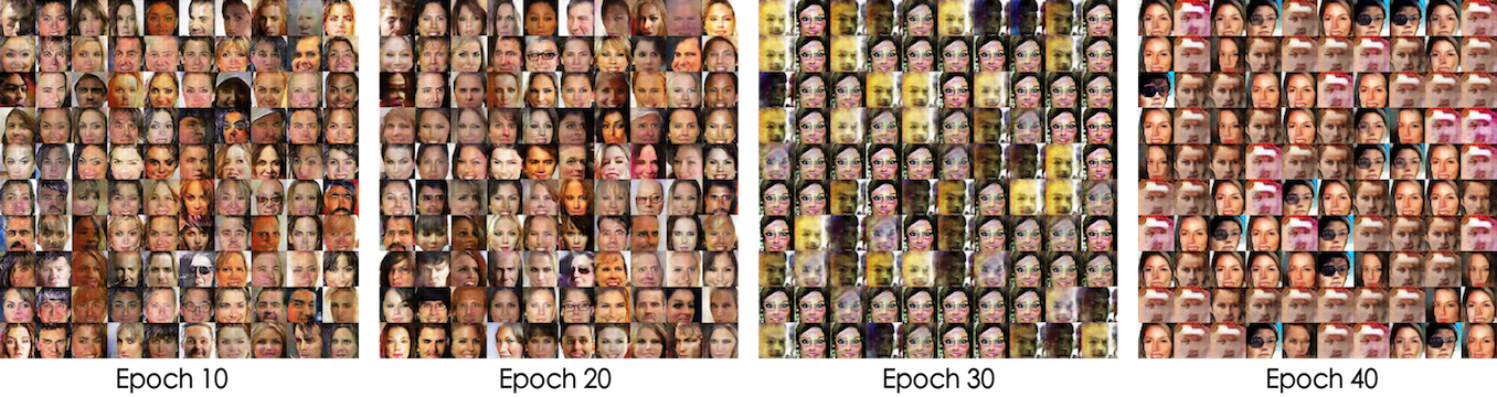
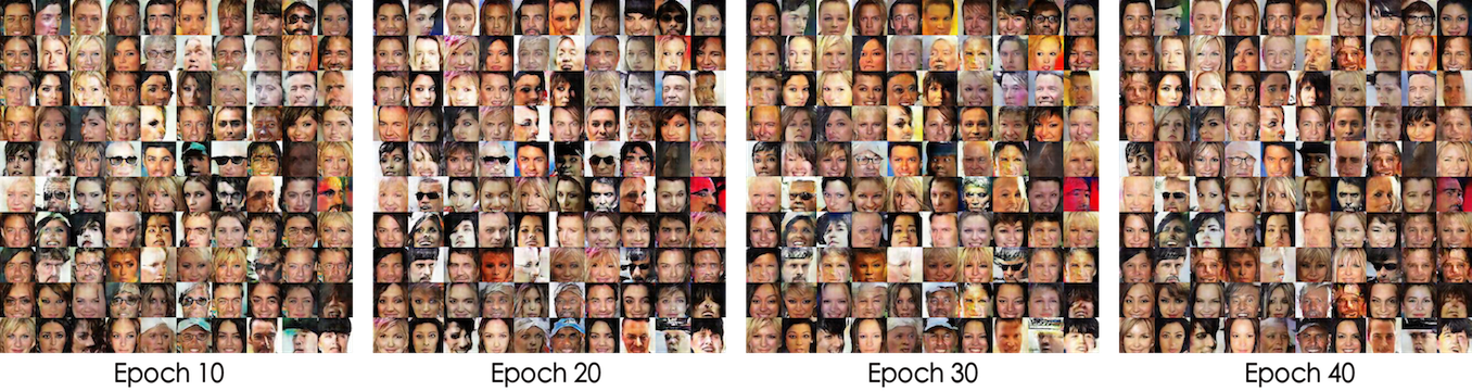
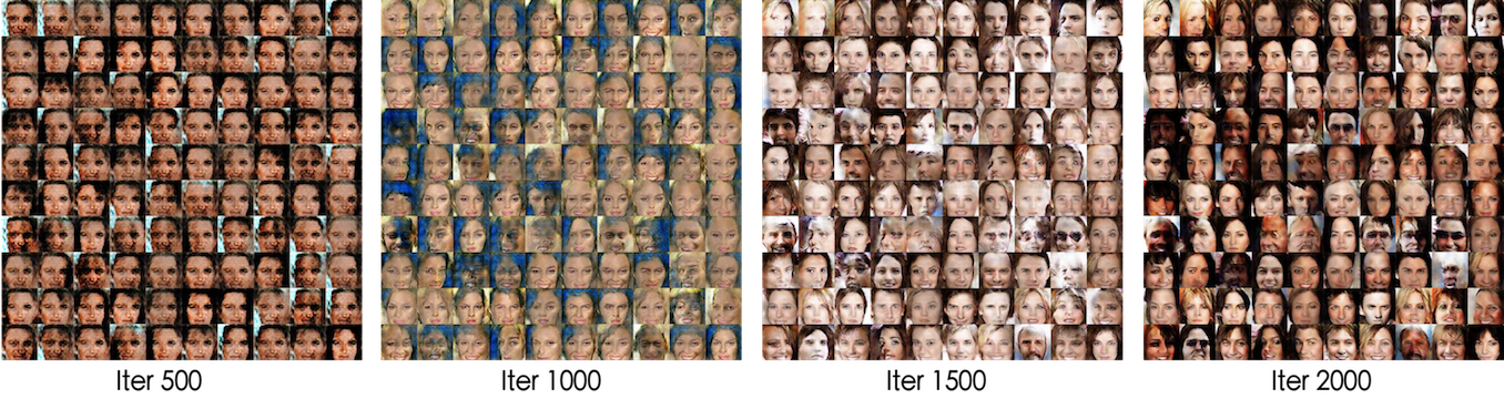
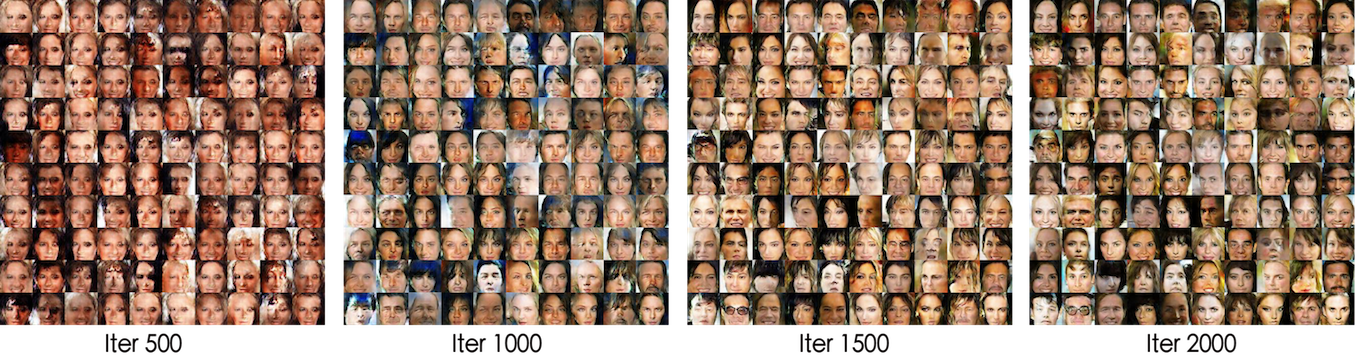
The following two experiments on the CelebA face dataset show that this regularization term is effective.

Experiment 1: Ordinary DCGAN network, training the generator and discriminator for one batch each per iteration.

Experiment 2: Ordinary DCGAN network, but with BN removed, training the generator and discriminator for five batches each per iteration.

AAE from a GAN Perspective

In fact, simply swapping the positions of x and z in the GAN discussion yields the AAE framework.

Specifically, AAE hopes to train an encoding model p(z|x) to map the true distribution \tilde{q}(x) to a standard Gaussian distribution q(z)=N(z;0,I), where: p(z|x)=\delta\left(z - E(x)\right),\quad p(z)=\int p(z|x)\tilde{q}(x)dx and E(x) is the neural network of the encoder.

Like GAN, AAE introduces a binary latent variable y, and has: p(z,y)=\left\{\begin{aligned}&p(z)p_1,\,y=1\\&q(z)p_0,\,y=0\end{aligned}\right. Similarly, we take p_1=p_0=1/2. On the other hand, we set q(z,y)=q(y|z) q(z), where the posterior distribution p(y|z) is a binary distribution with input z, and then optimize KL\left(p(z,y)\Vert q(z,y) \right): \begin{aligned} KL\left(p(z,y)\Vert q(z,y) \right)&=\int p(z)p_1\log \frac{p(z)p_1}{q(1|z)q(z)}dz+\int q(z)p_0\log \frac{q(z)p_0}{q(0|z)q(z)}dz\\ &\sim\int p(z)\log \frac{p(z)}{q(1|z)q(z)}dz+\int q(z)\log \frac{1}{q(0|z)}dz \end{aligned}

Now our optimization targets are q(y|z) and E(x). Let q(0|z)=D(z), and again perform alternating optimization: first fix E(x), which means p(z) is fixed, and then optimize q(y|z). Omitting constants, the optimization objective is: \begin{aligned} D=\mathop{\text{argmin}}_D &-\mathbb{E}_{z\sim p(z)}\left[\log (1-D(z))\right]-\mathbb{E}_{z\sim q(z)}\left[\log D(z)\right]\\ =\mathop{\text{argmin}}_D &-\mathbb{E}_{x\sim \tilde{p}(x)}\left[\log (1-D(E(x)))\right]-\mathbb{E}_{z\sim q(z)}\left[\log D(z)\right] \end{aligned} Then fix D(z) to optimize E(x). The relevant loss is: E = \mathop{\text{argmin}}_E \int p(z)\log \frac{p(z) }{(1-D(z)) q(z)}dz Using the theoretical optimal solution for D(z), D(z)=q(z)/[p^{o}(z)+q(z)], and substituting it into the loss, we get: \mathbb{E}_{x\sim \tilde{p}(x)}[-\log D(E(x))] + KL\left(p(z)\Vert p^{o}(z)\right) On one hand, like standard GAN, with careful training, we can remove the second term to get: \mathbb{E}_{x\sim \tilde{p}(x)}[-\log D(E(x))] On the other hand, we can train a decoder G(z) after obtaining the encoder. If the fitting capacity of the assumed E(x) and G(z) is sufficient, the reconstruction error can be small enough, and adding G(z) to the above loss will not interfere with GAN training. Therefore, they can be trained jointly: G,E = \mathop{\text{argmin}}_{G,E}\mathbb{E}_{x\sim \tilde{p}(x)}\left[-\log D(E(x))+\lambda\Vert x - G(E(x))\Vert^2\right]

Counter-intuitive ALI Version

ALI is like a fusion of GAN and AAE; another almost identical work is Bidirectional GAN (BiGAN). Compared to GAN, it incorporates z as a latent variable into variational inference. Specifically, in ALI: q(x,z,y)=\left\{\begin{aligned}&p(z|x)\tilde{p}(x) p_1,\,y=1\\&q(x|z)q(z)p_0,\,y=0\end{aligned}\right. and p(x,z,y)=p(y|x,z) p(z|x) \tilde{p}(x). Then optimize KL\left(q(x,z,y)\Vert p(x,z,y) \right): \begin{aligned} &\iint p(z|x)\tilde{p}(x) p_1\log \frac{p(z|x)\tilde{p}(x) p_1}{p(1|x,z) p(z|x) \tilde{p}(x)}dxdz\\ +&\iint q(x|z)q(z)p_0\log \frac{q(x|z)q(z)p_0}{p(0|x,z) p(z|x) \tilde{p}(x)}dxdz \end{aligned} This is equivalent to minimizing: \label{eq:ori-loss-ali} \iint p(z|x)\tilde{p}(x)\log \frac{1}{p(1|x,z)}dxdz+\iint q(x|z)q(z)\log \frac{q(x|z)q(z)}{p(0|x,z) p(z|x) \tilde{p}(x)}dxdz Now the optimization targets are p(y|x,z), p(z|x), q(x|z). Let p(1|x,z)=D(x,z). Again, perform alternating optimization: first fix E, G, then the loss related to D is: D=\mathop{\text{argmin}}_D -\mathbb{E}_{x\sim\tilde{p}(x),z\sim p(z|x)} \log D(x,z) - \mathbb{E}_{z\sim q(z),x\sim q(x|z)} \log (1-D(x,z)) Next, fix D to optimize G, E. Using the optimal solution for D: D(x,z)=\frac{p^{o}(z|x)\tilde{p}(x)}{p^{o}(z|x)\tilde{p}(x)+q^{o}(x|z)q(z)} it can be transformed into: \begin{aligned} &-\iint p(z|x)\tilde{p}(x)\log D(x, z) dxdz -\iint q(x|z) q(z)\log D(x, z) dxdz\\ &+\int q(z) KL(q(x|z)\Vert q^o(x|z)) dz + \iint q(x|z) q(z)\log \frac{p^o(z|x)}{p(z|x)}dxdz \end{aligned} Like standard GAN, with careful training, we can simply remove the last two terms to get: \label{eq:our-ali-g} -\iint p(z|x)\tilde{p}(x)\log D(x, z) dxdz -\iint q(x|z) q(z)\log D(x, z) dxdz This is the loss for the ALI generator and encoder we derived, which differs from the standard ALI results. Standard ALI (including ordinary GAN) treats it as a minimax problem, so the loss for the generator and encoder is: \label{eq:our-ali-g-o1} \iint p(z|x)\tilde{p}(x)\log D(x, z) dxdz + \iint q(x|z) q(z)\log (1-D(x, z)) dxdz or: \label{eq:our-ali-g-o2} -\iint p(z|x)\tilde{p}(x)\log (1-D(x, z)) dxdz -\iint q(x|z) q(z)\log D(x, z) dxdz Neither is equivalent to [eq:our-ali-g].