SamplePairing and mixup are two image data augmentation techniques that share a common lineage. They appear quite counter-intuitive and are extremely simple to implement, yet the results are impressive: multiple image classification tasks have shown that they can improve the accuracy of the final classification models.
Some readers might be puzzled by a question: why do such seemingly unreasonable data augmentation methods yield such good results? This article aims to show that while they appear to be data augmentation methods, they are actually a form of regularization for the model. As a classic line from Stephen Chow’s movie From Beijing with Love goes:
On the surface, this is a hair dryer, but in fact, it is a razor.
Data Augmentation
Let’s start with data augmentation. Data augmentation refers to the idea that after applying simple transformations to original data, their corresponding categories usually do not change. Therefore, we can "create" more data based on the original data. For example, if we take a photo of a dog and apply operations like horizontal flipping, slight rotation, cropping, or translation, we believe its category remains unchanged—it is still the same dog. In this way, several samples can be derived from a single sample, thereby increasing the volume of training data.
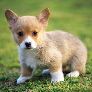
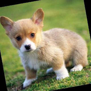
Data augmentation stems from our prior knowledge. For instance, we know beforehand that ordinary photos possess horizontal flip invariance, so we use horizontal flipping to augment data, telling the model through these augmented samples that it should possess horizontal flip invariance. Data augmentation is not universally applicable; for example, while ordinary photos can be horizontally flipped, text images cannot. This further illustrates that data augmentation is a scheme for integrating our prior knowledge into the model.
SamplePairing
Now let’s discuss SamplePairing. SamplePairing was proposed as a means of data augmentation, but it is highly counter-intuitive:
If the label of sample x_a is y_a, then randomly select a sample x_b from the training set, and let the label of (x_a + x_b)/2 still be y_a.
Yes, you read that correctly, and I didn’t write it wrong. It is that simple and that counter-intuitive. On paperweekly, reader Chen Taihong once commented:
This is the simplest paper I have ever seen in the CNN field.
Upon seeing this scheme, a series of questions might pop into a reader’s mind, which is exactly where the counter-intuitive nature of SamplePairing lies. For example, why is the label of (x_a + x_b)/2 assigned as y_a instead of y_b? Furthermore, according to our understanding of data augmentation, (x_a + x_b)/2 is no longer a "reasonable" image. Can such "augmentation" even be used?

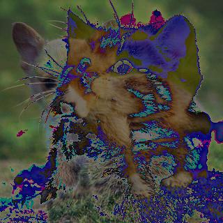
First, regarding the asymmetry: notice that when the current sample is x_a, we randomly pick x_b and set the label of (x_a + x_b)/2 to y_a. When it is x_b’s turn, the random selection might pick x_a, and then the label of (x_a + x_b)/2 becomes y_b. So, while it looks asymmetric, SamplePairing is actually symmetric in practice. SamplePairing can be reformulated as:
Randomly select two samples x_a and x_b with labels y_a and y_b. Randomly pick one of the labels, say y, and let the label of (x_a + x_b)/2 be y.
mixup
From the reformulated SamplePairing, it is not hard to see that if training is sufficient, the model’s output for (x_a + x_b)/2 should theoretically be half y_a and half y_b. That is to say, if y_a and y_b represent one-hot vectors for the categories, the output for (x_a + x_b)/2 should be (y_a + y_b)/2.
In that case, why not mix them in a more random way? Suppose U(\varepsilon) is some random distribution on [0, 1]. Each time, we randomly sample \varepsilon \sim U(\varepsilon), and then let the output corresponding to \varepsilon x_a + (1-\varepsilon) x_b be \varepsilon y_a + (1-\varepsilon) y_b. In the original paper, U(\varepsilon) is chosen as a \beta distribution, but I feel this introduces more hyperparameters; it might be simpler to just let it be a uniform distribution.
Compared to SamplePairing, the approach of mixup is "softer" and more convincing. SamplePairing often feels like an "all-or-nothing" approach, whereas mixup is more intuitive: since the input is superimposed in a ratio of \varepsilon : 1-\varepsilon, it is natural that the output should also be superimposed in the same way.
Regularization Interpretation
Although mixup feels more reasonable, neither method answers a crucial question: After adding two images together, the result is no longer a valid image. This is completely different from what we usually call data augmentation. Why does it still work?
Let’s describe this problem more mathematically. For a training set (x_1, y_1), (x_2, y_2), \dots, (x_n, y_n), we hope to find a model f such that y = f(x). For tasks like image classification, given the strong non-linearity of the problem itself, we generally use very deep networks to fit the data. However, a deeper network also means it is more prone to overfitting the training set.
Suppose the model already has the ability to predict y_a = f(x_a) and y_b = f(x_b). For mixup, it says this is not enough; the model must also output \varepsilon y_a + (1-\varepsilon) y_b for the input \varepsilon x_a + (1-\varepsilon) x_b. That is: \varepsilon y_a + (1-\varepsilon) y_b = f\big(\varepsilon x_a + (1-\varepsilon) x_b\big) Replacing y_a, y_b with f(x_a), f(x_b), we get: \varepsilon f(x_a) + (1-\varepsilon) f(x_b) = f\big(\varepsilon x_a + (1-\varepsilon) x_b\big) This is actually a functional equation. If \varepsilon, x_a, x_b are arbitrary, the solution to this functional equation is a "linear function." In other words, only a linear function can make the above equation hold identically. Put another way, mixup encourages the model f to be a linear function.
We know that a linear function is equivalent to a single-layer neural network without an activation function, which is arguably the simplest model. Our actual models are deep networks with a massive number of parameters and strong non-linear capabilities; the more parameters, the easier it is to overfit. Thus, the meaning of mixup becomes clear:
mixup acts as a regularization term. It encourages the model to stay as close to a linear function as possible. That is, it ensures the model’s predictions are as accurate as possible while keeping the model as simple as possible.
Therefore, mixup is a powerful model filter:
Among all models with similar performance, choose the one that is closest to a linear function.
Final Thoughts
We have now answered the original question: techniques like SamplePairing and mixup only wear the mask of data augmentation. In reality, they use the form of data augmentation to add a regularization term to the model, or in other words, to prune the model.
Therefore, we don’t need to agonize over the question of "why data augmentation is effective when the added images are no longer reasonable images," because it isn’t actually data augmentation.
Finally, I’ll conclude this article by playfully adapting a poem by Tang Bohu:
Others laugh at my random augmentations, I laugh at others for not seeing through.
No reasonable images emerge, yet the model is filtered silently.
Original Address: https://kexue.fm/archives/5693
For more details on reprinting, please refer to: Scientific Space FAQ