Originally, I had decided not to play with RNNs anymore. However, while reflecting last week, I suddenly realized that RNNs actually correspond to numerical methods for solving ODEs (Ordinary Differential Equations). This provided a path for something I have always wanted to do: using deep learning to solve pure mathematical problems. In fact, this is a rather interesting and useful result, so I will introduce it here. Incidentally, this article also involves writing your own RNNs from scratch, so it can serve as a simple tutorial for creating custom RNN layers.
Note: This article is not an introduction to the recent trending topic "Neural ODEs" (though there is a certain connection).
RNN Basics
What is an RNN?
As is well known, RNN stands for "Recurrent Neural Network." Unlike CNNs, an RNN is a general term for a class of models rather than a single specific model. Simply put, any model that takes an input vector sequence (\boldsymbol{x}_1, \boldsymbol{x}_2, \dots, \boldsymbol{x}_T), produces another vector sequence (\boldsymbol{y}_1, \boldsymbol{y}_2, \dots, \boldsymbol{y}_T), and satisfies the following recursive relationship: \boldsymbol{y}_t = f(\boldsymbol{y}_{t-1}, \boldsymbol{x}_t, t) \tag{1} can be called an RNN. Because of this, the original vanilla RNN, as well as improved models like GRU, LSTM, and SRU, are all called RNNs because they can be seen as special cases of the above equation. There are also some things that seem unrelated to RNNs, such as the calculation of the CRF denominator introduced recently, which is actually a simple RNN.
To put it plainly, RNN is essentially recursive computation.
Writing Your Own RNN
Here we first introduce how to use Keras to quickly and easily write a custom RNN.
In fact, whether in Keras or pure TensorFlow, customizing your own
RNN is not complicated. In Keras, you just need to write the recursive
function for each step; in TensorFlow, it is slightly more complex,
requiring you to encapsulate the recursive function into an
RNNCell class. Below is an implementation of a basic RNN in
Keras: \boldsymbol{y}_t =
\tanh(\boldsymbol{W}_1 \boldsymbol{y}_{t-1} + \boldsymbol{W}_2
\boldsymbol{x}_t + \boldsymbol{b}) \tag{2} The code is very
simple:
#! -*- coding: utf-8- -*-

from keras.layers import Layer
import keras.backend as K

class My_RNN(Layer):

    def __init__(self, output_dim, **kwargs):
        self.output_dim = output_dim # Output dimension
        super(My_RNN, self).__init__(**kwargs)

    def build(self, input_shape): # Define trainable parameters
        self.kernel1 = self.add_weight(name='kernel1',
                                      shape=(self.output_dim, self.output_dim),
                                      initializer='glorot_normal',
                                      trainable=True)
        self.kernel2 = self.add_weight(name='kernel2',
                                      shape=(input_shape[-1], self.output_dim),
                                      initializer='glorot_normal',
                                      trainable=True)
        self.bias = self.add_weight(name='bias',
                                      shape=(self.output_dim,),
                                      initializer='glorot_normal',
                                      trainable=True)

    def step_do(self, step_in, states): # Define iteration for each step
        step_out = K.tanh(K.dot(states[0], self.kernel1) +
                          K.dot(step_in, self.kernel2) +
                          self.bias)
        return step_out, [step_out]

    def call(self, inputs): # Define the execution function
        init_states = [K.zeros((K.shape(inputs)[0],
                                self.output_dim)
                              )] # Define initial state (all zeros)
        outputs = K.rnn(self.step_do, inputs, init_states) # Loop step_do
        return outputs[0] # outputs is a tuple, outputs[0] is the last output,
                          # outputs[1] is the full sequence, output[2] is a list
                          # of intermediate hidden states.

    def compute_output_shape(self, input_shape):
        return (input_shape[0], self.output_dim)
As you can see, although there are many lines of code, most are
boilerplate. What truly defines the RNN is
the step_do function. This function accepts two inputs:
step_in and states. step_in is a
tensor of shape (batch_size, input_dim) representing the
current sample \boldsymbol{x}_t, while
states is a list representing \boldsymbol{y}_{t-1} and some intermediate
variables. It is important to note that states is a list of
tensors, not a single tensor, because multiple intermediate variables
might need to be passed during recursion (e.g., LSTM requires two state
tensors). Finally, step_do must return \boldsymbol{y}_t and the new
states; this is the standard for writing this
function.
The K.rnn function accepts
three basic parameters: the first is the step_do function
we just wrote, the second is the input time series, and the third is the
initial state, which matches the states mentioned earlier.
Naturally, init_states is also a list of tensors, usually
initialized to all zeros.
ODE Basics
What is an ODE?
ODE stands for "Ordinary Differential Equation." Here we refer to a general system of ordinary differential equations: \dot{\boldsymbol{x}}(t) = \boldsymbol{f}\big(\boldsymbol{x}(t), t\big) \tag{3} The field studying ODEs is often directly called "Dynamics" or "Dynamical Systems," because Newtonian mechanics is usually just a set of ODEs.
ODEs can generate a very rich variety of functions. For example, e^t is the solution to \dot{x}=x, and \sin t and \cos t are solutions to \ddot{x}+x=0 (with different initial conditions). In fact, some tutorials define the e^t function directly through the differential equation \dot{x}=x. Besides these elementary functions, many special functions whose names we know but whose natures seem mysterious are derived via ODEs, such as hypergeometric functions, Legendre functions, Bessel functions...
In short, ODEs can and do generate all sorts of strange and wonderful functions.
Numerical Solutions to ODEs
ODEs that can be solved exactly with analytical solutions are quite rare, so we often require numerical methods.
Numerical solutions for ODEs are a mature discipline. We won’t introduce much here, only the most basic iteration formula proposed by the mathematician Euler: \boldsymbol{x}(t + h) = \boldsymbol{x}(t) + h \boldsymbol{f}\big(\boldsymbol{x}(t), t\big) \tag{4} where h is the step size. Euler’s method comes from a simple approximation: \frac{\boldsymbol{x}(t + h) - \boldsymbol{x}(t)}{h} \tag{5} to approximate the derivative term \dot{\boldsymbol{x}}(t). Given an initial condition \boldsymbol{x}(0), we can iterate step-by-step using (4) to calculate the result at each time point.
ODE and RNN
ODEs are also RNNs
If you compare (4) and (1) carefully, do you see the connection?
In (1), t is an integer variable, while in (4), t is a floating-point variable. Other than that, there is no obvious difference between (4) and (1). In fact, in (4), we can use h as the unit of time and let t=nh, then (4) becomes: \boldsymbol{x}\big((n+1)h\big) = \boldsymbol{x}(nh) + h \boldsymbol{f}\big(\boldsymbol{x}(nh), nh\big) \tag{6} Now the time variable n in (6) is also an integer.
Thus, we know: Euler’s method for ODEs (4) is actually just a special case of an RNN. This might indirectly explain why RNNs have such strong fitting capabilities (especially for time-series data). We see that ODEs can generate many complex functions, and since an ODE is just a special case of an RNN, RNNs can generate even more complex functions.
Solving ODEs with RNNs
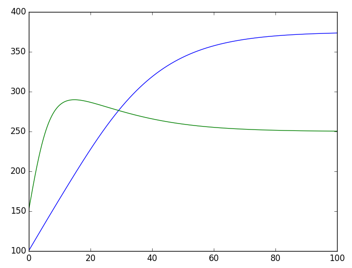
Consequently, we can write an RNN to solve an ODE. For example, take the case from "Competition Model of Two Biological Populations": \left\{\begin{aligned}\frac{dx_1}{dt}=r_1 x_1\left(1-\frac{x_1}{N_1}\right)-a_1 x_1 x_2 \\ \frac{dx_2}{dt}=r_2 x_2\left(1-\frac{x_2}{N_2}\right)-a_2 x_1 x_2\end{aligned}\right. \tag{7} We can write:
#! -*- coding: utf-8- -*-

from keras.layers import Layer
import keras.backend as K

class ODE_RNN(Layer):

    def __init__(self, steps, h, **kwargs):
        self.steps = steps
        self.h = h
        super(ODE_RNN, self).__init__(**kwargs)

    def step_do(self, step_in, states): # Define iteration for each step
        x = states[0]
        r1,r2,a1,a2,iN1,iN2 = 0.1,0.3,0.0001,0.0002,0.002,0.003
        _1 = r1 * x[:,0] * (1 - iN1 * x[:,0]) - a1 * x[:,0] * x[:,1]
        _2 = r2 * x[:,1] * (1 - iN2 * x[:,1]) - a2 * x[:,0] * x[:,1]
        _1 = K.expand_dims(_1, 1)
        _2 = K.expand_dims(_2, 1)
        _ = K.concatenate([_1, _2], 1)
        step_out = x + self.h * _
        return step_out, [step_out]

    def call(self, inputs): # inputs are the initial conditions
        init_states = [inputs]
        zeros = K.zeros((K.shape(inputs)[0],
                         self.steps,
                         K.shape(inputs)[1])) # No external input needed
                                              # dummy zeros for K.rnn
        outputs = K.rnn(self.step_do, zeros, init_states)
        return outputs[1] # Output the entire sequence

    def compute_output_shape(self, input_shape):
        return (input_shape[0], self.steps, input_shape[1])

from keras.models import Sequential
import numpy as np
import matplotlib.pyplot as plt

steps, h = 1000, 0.1

M = Sequential()
M.add(ODE_RNN(steps, h, input_shape=(2,)))
M.summary()

# Forward propagation directly outputs the solution
result = M.predict(np.array([[100, 150]]))[0] # Initial condition [100, 150]
times = np.arange(1, steps+1) * h

# Plotting
plt.plot(times, result[:,0])
plt.plot(times, result[:,1])
plt.savefig('test.png')
The process is easy to understand, but two points should be noted.
First, since the system of equations (7) is only two-dimensional and not
easily written as matrix operations, I operated on the indices directly
in the step_do function (x[:,0], x[:,1]). If
the equation had higher dimensions and could be written as matrix
operations, it would be more efficient. Second, after building the
model, calling predict outputs the result directly; no
"training" is required.
Inferring ODE Parameters
The previous section showed that the forward propagation of an RNN corresponds to the Euler solution of an ODE. What does backpropagation correspond to?
In practical problems, there is a class of problems called "model inference," which involves guessing the model (mechanism inference) that fits a set of experimental data. This usually involves two steps: first, guessing the form of the model, and second, determining the model’s parameters. Assuming the data can be described by an ODE and the form of the ODE is known, we need to estimate the parameters within it.
If the ODE could be solved analytically, this would be a simple regression problem. But as mentioned, most ODEs have no closed-form solution, so numerical methods are necessary. This is exactly what backpropagation in the corresponding RNN does: forward propagation solves the ODE (the RNN’s prediction process), and backpropagation naturally infers the ODE’s parameters (the RNN’s training process). This is a very interesting fact: ODE parameter inference is a well-studied subject, yet in deep learning, it is just a basic application of RNNs.
Let’s save the solution data from the previous example and take only a few points to see if we can reverse-engineer the original differential equation. The data points are:
| Time | 0 | 10 | 15 | 30 | 36 | 40 | 42 |
|---|---|---|---|---|---|---|---|
| x_1 | 100 | 165 | 197 | 280 | 305 | 318 | 324 |
| x_2 | 150 | 283 | 290 | 276 | 269 | 266 | 264 |
Assuming we only know these limited data points and the form of equation (7), we want to find the parameters. We modify the previous code:
#! -*- coding: utf-8- -*-

from keras.layers import Layer
import keras.backend as K

def my_init(shape, dtype=None): # Need proper initialization
    return K.variable([0.1, 0.1, 0.001, 0.001, 0.001, 0.001])

class ODE_RNN(Layer):

    def __init__(self, steps, h, **kwargs):
        self.steps = steps
        self.h = h
        super(ODE_RNN, self).__init__(**kwargs)

    def build(self, input_shape): # Set parameters as trainable
        self.kernel = self.add_weight(name='kernel',
                                      shape=(6,),
                                      initializer=my_init,
                                      trainable=True)
    def step_do(self, step_in, states):
        x = states[0]
        r1,r2,a1,a2,iN1,iN2 = (self.kernel[0], self.kernel[1],
                               self.kernel[2], self.kernel[3],
                               self.kernel[4], self.kernel[5])
        _1 = r1 * x[:,0] * (1 - iN1 * x[:,0]) - a1 * x[:,0] * x[:,1]
        _2 = r2 * x[:,1] * (1 - iN2 * x[:,1]) - a2 * x[:,0] * x[:,1]
        _1 = K.expand_dims(_1, 1)
        _2 = K.expand_dims(_2, 1)
        _ = K.concatenate([_1, _2], 1)
        step_out = x + self.h * K.clip(_, -1e5, 1e5) # Prevent gradient explosion
        return step_out, [step_out]

    def call(self, inputs):
        init_states = [inputs]
        zeros = K.zeros((K.shape(inputs)[0],
                         self.steps,
                         K.shape(inputs)[1]))
        outputs = K.rnn(self.step_do, zeros, init_states)
        return outputs[1]

    def compute_output_shape(self, input_shape):
        return (input_shape[0], self.steps, input_shape[1])

from keras.models import Sequential
from keras.optimizers import Adam
import numpy as np
import matplotlib.pyplot as plt

steps, h = 50, 1 # Large step size to reduce steps and long-term dependency
series = {0: [100, 150],
          10: [165, 283],
          15: [197, 290],
          30: [280, 276],
          36: [305, 269],
          40: [318, 266],
          42: [324, 264]}

M = Sequential()
M.add(ODE_RNN(steps, h, input_shape=(2,)))
M.summary()

# Construct training samples
X = np.array([series[0]])
Y = np.zeros((1, steps, 2))

for i,j in series.items():
    if i != 0:
        Y[0, int(i/h)-1] += series[i]

# Custom loss: only consider time points where data exists
def ode_loss(y_true, y_pred):
    T = K.sum(K.abs(y_true), 2, keepdims=True)
    T = K.cast(K.greater(T, 1e-3), 'float32')
    return K.sum(T * K.square(y_true - y_pred), [1, 2])

M.compile(loss=ode_loss, optimizer=Adam(1e-4))
M.fit(X, Y, epochs=10000)

# Predict and plot
result = M.predict(np.array([[100, 150]]))[0]
times = np.arange(1, steps+1) * h

plt.clf()
plt.plot(times, result[:,0], color='blue')
plt.plot(times, result[:,1], color='green')
plt.plot(list(series.keys()), [i[0] for i in series.values()], 'o', color='blue')
plt.plot(list(series.keys()), [i[1] for i in series.values()], 'o', color='green')
plt.savefig('test.png')
The results can be seen in the following figure:

Clearly, the results are satisfying.
Conclusion
This article introduced the RNN model and its custom implementation in Keras within a general framework, then revealed the connection between ODEs and RNNs. Based on this, it introduced the basic ideas of solving ODEs directly with RNNs and inferring ODE parameters using RNNs. I must remind readers that in the backpropagation of RNN models, one must be cautious with initialization and truncation, and choose the learning rate carefully to prevent gradient explosion (gradient vanishing is just poor optimization, but gradient explosion leads to total collapse; solving gradient explosion is particularly important).
In short, gradient vanishing and explosion are classic difficulties
in RNNs. In fact, models like LSTM and GRU were introduced primarily to
solve the gradient vanishing problem, while gradient explosion is
addressed by using tanh or sigmoid activation
functions. However, if we use RNNs to solve ODEs, we do not have the
freedom to choose activation functions (the activation function is part
of the ODE itself), so we must be careful with initialization and other
treatments. It is said that as long as initialization is done carefully,
using ReLU as an activation function in a standard RNN is perfectly
fine.
When reposting, please include the original article address: https://kexue.fm/archives/5643
For more detailed reposting matters, please refer to: "Scientific Space FAQ"