Due to professional requirements, I needed to perform stochastic simulation of the Master Equation. I couldn’t find a suitable Python implementation online, so I wrote one myself and am sharing the source code here. As for the Gillespie algorithm itself, I will not introduce it; readers who need it will naturally understand, and those who do not are advised not to bother.
Source Code
In fact, the basic Gillespie simulation algorithm is very simple and easy to implement. Below is a reference example:
#! -*- coding: utf-8 -*-

import numpy as np
from scipy.special import comb

class Reaction: # Encapsulated class representing each chemical reaction
    def __init__(self, rate=0., num_lefts=None, num_rights=None):
        self.rate = rate # Reaction rate
        assert len(num_lefts) == len(num_rights)
        self.num_lefts = np.array(num_lefts) # Number of each reactant before reaction
        self.num_rights = np.array(num_rights) # Number of each reactant after reaction
        self.num_diff = self.num_rights - self.num_lefts # Change in number
    def combine(self, n, s): # Calculate combinations
        return np.prod(comb(n, s))
    def propensity(self, n): # Calculate propensity function
        return self.rate * self.combine(n, self.num_lefts)

class System: # Encapsulated class representing a system of multiple reactions
    def __init__(self, num_elements):
        assert num_elements > 0
        self.num_elements = num_elements # Number of species in the system
        self.reactions = [] # Set of reactions
    def add_reaction(self, rate=0., num_lefts=None, num_rights=None):
        assert len(num_lefts) == self.num_elements
        assert len(num_rights) == self.num_elements
        self.reactions.append(Reaction(rate, num_lefts, num_rights))
    def evolute(self, steps, inits=None): # Simulate evolution
        self.t = [0] # Time trajectory, t[0] is initial time
        if inits is None:
            self.n = [np.ones(self.num_elements)]
        else:
            self.n = [np.array(inits)] # Reactant counts, n[0] is initial count
        for i in range(steps):
            A = np.array([rec.propensity(self.n[-1])
                          for rec in self.reactions]) # Propensity for each reaction
            A0 = A.sum()
            A /= A0 # Normalize to get probability distribution
            t0 = -np.log(np.random.random())/A0 # Time interval to next reaction
            self.t.append(self.t[-1] + t0)
            d = np.random.choice(self.reactions, p=A) # Choose one reaction to occur
            self.n.append(self.n[-1] + d.num_diff)
Usage
For convenience, I have encapsulated the reactions. Now, you can perform simulations directly based on the reaction equations without additional programming. For example, consider a simple gene expression model:
\begin{aligned} DNA &\xrightarrow{\quad 20\quad} DNA + m\\ m &\xrightarrow{\quad 2.5\quad} m + n\\ m &\xrightarrow{\,\quad 1\,\,\quad} \phi\\ n &\xrightarrow{\,\quad 1\,\,\quad} \phi \end{aligned}
Here m and n represent the counts of mRNA and protein, respectively, and \phi represents the empty set, implying degradation or "creation from nothing." The first reaction can be simplified to \phi \xrightarrow{\quad 20\quad} m, so it is actually four reaction equations involving two species m and n.
num_elements = 2
system = System(num_elements)

system.add_reaction(20, [0, 0], [1, 0])
system.add_reaction(2.5, [1, 0], [1, 1])
system.add_reaction(1, [1, 0], [0, 0])
system.add_reaction(1, [0, 1], [0, 0])

system.evolute(100000)
Then you can perform statistics and plotting:
import matplotlib.pyplot as plt
import pandas as pd

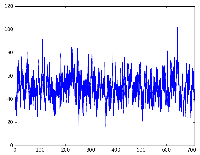
x = system.t
y = [i[1] for i in system.n]

plt.clf()
plt.plot(x, y) # Trajectory plot of protein
plt.xlim(0, x[-1]+1)
plt.savefig('test.png')

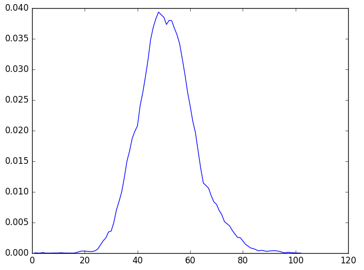
d = pd.Series([i[1] for i in system.n]).value_counts()
d = d.sort_index()
d /= d.sum()
plt.clf()
plt.plot(d.index, d) # (Empirical) distribution plot of protein
plt.savefig('test.png')
The results are:
When reposting, please include the original address of
this article:
https://kexue.fm/archives/5607
For more detailed information regarding reposting, please
refer to:
"Scientific Space FAQ"