A Concise Introduction to Conditional Random Fields (CRF) (with a Pure Keras Implementation)

Frame-wise Softmax

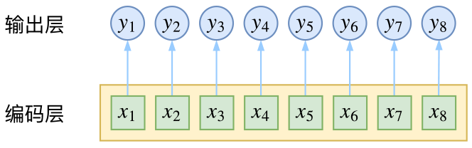
CRF is primarily used for sequence labeling problems, which can be simply understood as classifying every frame in a sequence. Since it is a classification task, a natural idea is to encode the sequence using a CNN or RNN and then connect it to a fully connected layer with softmax activation, as shown in the figure below:

Conditional Random Fields

However, when we design labels—for example, using the four labels s, b, m, e for character-based word segmentation—the target output sequence itself carries certain contextual correlations. For instance, s cannot be followed by m or e, and so on. Frame-wise softmax does not consider these output-level contextual correlations, which means it delegates these correlations to the encoding layer, hoping the model can learn them on its own. Sometimes, this "asks too much of the model."

CRF is more direct: it separates the output-level correlations, which allows the model to be more "composed" during learning:

Model Overview

Suppose an input has n frames and each frame has k possible labels. Theoretically, there are k^n different possible outputs. We can visualize this using the network diagram below. In the diagram, each point represents a possible label, the lines between points represent the associations between labels, and every labeling result corresponds to a complete path through the graph.

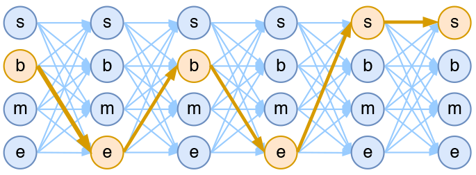
In sequence labeling tasks, our correct answer is generally unique. For example, for "Today’s weather is good," if the segmentation result is "Today / weather / is / good," the target output sequence would be bebebe (assuming a specific tagging scheme). No other path satisfies the requirement. In other words, in sequence labeling tasks, our basic unit of study should be the path. What we need to do is select the correct one from k^n paths. This means that if we view it as a classification problem, it is a classification problem of choosing one class out of k^n classes!

This is the fundamental difference between frame-wise softmax and CRF: the former treats sequence labeling as n k-classification problems, while the latter treats it as a single k^n-classification problem.

Specifically, in the CRF sequence labeling problem, we want to calculate the conditional probability: P(y_1,\dots,y_n|x_1,\dots,x_n)=P(y_1,\dots,y_n|\boldsymbol{x}),\quad \boldsymbol{x}=(x_1,\dots,x_n) \tag{1} To estimate this probability, CRF makes two assumptions:

Assumption 1: The distribution belongs to the exponential family.

This assumption implies the existence of a function f(y_1,\dots,y_n;\boldsymbol{x}) such that: P(y_1,\dots,y_n|\boldsymbol{x})=\frac{1}{Z(\boldsymbol{x})}\exp\Big(f(y_1,\dots,y_n;\boldsymbol{x})\Big) \tag{2} where Z(\boldsymbol{x}) is the normalization factor (partition function). Since this is a conditional distribution, the normalization factor depends on \boldsymbol{x}. The function f can be viewed as a scoring function. The probability distribution is obtained by taking the exponential of the score and normalizing it.

Assumption 2: Correlations between outputs occur only at adjacent positions, and the correlations are additive in the exponent.

This assumption means f(y_1,\dots,y_n;\boldsymbol{x}) can be further simplified as: \begin{aligned} f(y_1,\dots,y_n;\boldsymbol{x})=&h(y_1;\boldsymbol{x})+g(y_1,y_2;\boldsymbol{x})+h(y_2;\boldsymbol{x})+g(y_2,y_3;\boldsymbol{x})+h(y_3;\boldsymbol{x})\\ &+\dots+g(y_{n-1},y_n;\boldsymbol{x})+h(y_n;\boldsymbol{x}) \end{aligned} \tag{3} This means we only need to score each label and each pair of adjacent labels separately, and then sum all the scores to get the total score.

Linear Chain CRF

Despite the significant simplifications, the probability model represented by Equation (3) is generally still too complex to solve. Considering that in current deep learning models, RNNs or stacked CNNs are already capable of capturing the relationship between each y and the input \boldsymbol{x} sufficiently, we might as well assume that the function g is independent of \boldsymbol{x}: \begin{aligned} f(y_1,\dots,y_n;\boldsymbol{x})=h(y_1;\boldsymbol{x})+&g(y_1,y_2)+h(y_2;\boldsymbol{x})+\dots\\ +&g(y_{n-1},y_n)+h(y_n;\boldsymbol{x}) \end{aligned} \tag{4} In this case, g is actually just a finite, trainable parameter matrix, and the single-label scoring function h(y_i;\boldsymbol{x}) can be modeled via an RNN or CNN. Thus, the model can be established, where the probability distribution becomes: P(y_1,\dots,y_n|\boldsymbol{x})=\frac{1}{Z(\boldsymbol{x})}\exp\left(h(y_1;\boldsymbol{x})+\sum_{t=1}^{n-1}\Big[g(y_t,y_{t+1})+h(y_{t+1};\boldsymbol{x})\Big]\right) \tag{5} This is the concept of a Linear Chain CRF.

Normalization Factor

To train the CRF model, we use the maximum likelihood method, which means using: -\log P(y_1,\dots,y_n|\boldsymbol{x}) \tag{6} as the loss function. It can be calculated as: -\left(h(y_1;\boldsymbol{x})+\sum_{t=1}^{n-1}\Big[g(y_t,y_{t+1})+h(y_{t+1};\boldsymbol{x})\Big]\right)+\log Z(\boldsymbol{x}) \tag{7} The first term is the logarithm of the numerator of the original probability expression, which is the score of the target sequence. Although it looks circuitous, it is not difficult to calculate. The real difficulty lies in the logarithm of the denominator, \log Z(\boldsymbol{x}).

The normalization factor, also called the partition function in physics, requires us to sum the exponents of the scores of all possible paths. As mentioned earlier, the number of such paths is exponential (k^n), making direct calculation nearly impossible.

In fact, the difficulty of calculating the normalization factor is a common challenge for almost all probabilistic graphical models. Fortunately, in the CRF model, because we only consider the relationship between adjacent labels (the Markov assumption), we can calculate the normalization factor recursively. This reduces the computational complexity from exponential to linear. Specifically, let Z_t be the normalization factor calculated up to time t, and divide it into k parts: Z_t = Z^{(1)}_t + Z^{(2)}_t + \dots + Z^{(k)}_t \tag{8} where Z^{(1)}_t,\dots,Z^{(k)}_t are the sums of the score exponents of all paths ending with labels 1,\dots,k at the current time t. Then, we can calculate recursively: \begin{aligned} Z^{(1)}_{t+1} = & \Big(Z^{(1)}_t G_{11} + Z^{(2)}_t G_{21} + \dots + Z^{(k)}_t G_{k1} \Big) H_{t+1}(1|\boldsymbol{x})\\ Z^{(2)}_{t+1} = & \Big(Z^{(1)}_t G_{12} + Z^{(2)}_t G_{22} + \dots + Z^{(k)}_t G_{k2} \Big) H_{t+1}(2|\boldsymbol{x})\\ & \qquad\qquad\vdots\\ Z^{(k)}_{t+1} = & \Big(Z^{(1)}_t G_{1k} + Z^{(2)}_t G_{2k} + \dots + Z^{(k)}_t G_{kk} \Big) H_{t+1}(k|\boldsymbol{x}) \end{aligned} \tag{9} This can be written simply in matrix form: \boldsymbol{Z}_{t+1} = \boldsymbol{Z}_{t} \boldsymbol{G} \otimes H(y_{t+1}|\boldsymbol{x}) \tag{10} where \boldsymbol{Z}_{t}=\Big[Z^{(1)}_t,\dots,Z^{(k)}_t\Big]; \boldsymbol{G} is the matrix obtained by taking the exponent of each element in the matrix g (as mentioned, in the simplest case, g is just a matrix representing the score of transitioning from one label to another), i.e., \boldsymbol{G}_{ij}=e^{g_{ij}}; and H(y_{t+1}|\boldsymbol{x}) is the exponent of the scores for each label at position t+1 from the encoding model h(y_{t+1}|\boldsymbol{x}) (RNN, CNN, etc.), i.e., H(y_{t+1}|\boldsymbol{x})=e^{h(y_{t+1}|\boldsymbol{x})}, which is also a vector. In Equation (10), \boldsymbol{Z}_{t} \boldsymbol{G} is a matrix multiplication resulting in a vector, and \otimes denotes element-wise multiplication of two vectors.

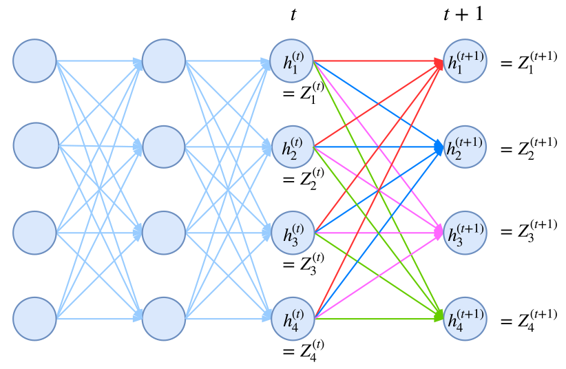
Readers unfamiliar with this might find Equation (10) difficult to accept at first. You can try writing out the normalization factors for n=1, n=2, n=3 and look for their recursive relationships to gradually understand it.

Dynamic Programming

Once the loss function -\log P(y_1,\dots,y_n|\boldsymbol{x}) is defined, model training can be completed. Since modern deep learning frameworks already include automatic differentiation, as long as we can write a differentiable loss, the framework will handle the optimization process.

The final step is to find the optimal path for a given input after the model is trained. As before, this is a problem of selecting the best path from k^n possibilities. Similarly, due to the Markov assumption, this can be transformed into a dynamic programming problem solved by the Viterbi algorithm, with a computational complexity proportional to n.

Dynamic programming has appeared many times in this blog. Its recursive idea is: if an optimal path is cut into two segments, then each segment is also a (locally) optimal path. You can find many related introductions by searching "dynamic programming" in the search box on the right side of this blog, so I won’t repeat it here.

Implementation Key Points

As explained earlier, the difficulty in implementing CRF is the calculation of -\log P(y_1,\dots,y_n|\boldsymbol{x}), and the core difficulty is the calculation of the normalization factor Z(\boldsymbol{x}). Thanks to the Markov assumption, we obtained the recursive Equation (9) or (10), which should be the standard way to calculate Z(\boldsymbol{x}) in general cases.

So, how do we implement this recursive calculation in a deep learning framework? Note that from a computational graph perspective, this defines a graph through recursion, and the length of this graph is not fixed. This shouldn’t be a problem for dynamic graph frameworks like PyTorch, but it is difficult for static graph frameworks like TensorFlow or Keras.

However, it is not impossible. We can use the built-in RNN functions for the calculation! We know that an RNN essentially performs a recursive calculation: \boldsymbol{h}_{t+1} = f(\boldsymbol{x}_{t+1}, \boldsymbol{h}_{t}) \tag{11} Newer versions of TensorFlow and Keras allow us to define custom RNN cells. This means the function f can be defined by us, and the backend will automatically handle the recursive calculation. Thus, we only need to design an RNN such that the \boldsymbol{Z} we want to calculate corresponds to the RNN’s hidden vector!

This is the most elegant part of the CRF implementation.

As for the rest, there are some technical details:

1. To prevent overflow, we usually work in the log domain. Since the normalization factor is a sum of exponents, it takes the form \log\left(\sum_{i=1}^k e^{a_i}\right). The trick for this calculation is: \log\left(\sum_{i=1}^k e^{a_i}\right)=A + \log\left(\sum_{i=1}^k e^{a_i-A}\right),\quad A = \max \{a_1,\dots,a_k\} TensorFlow and Keras already have the logsumexp function encapsulated; we can just call it.

2. For the calculation of the numerator (the score of the target sequence), the trick used in the code is to use the "target sequence" dot-product with the "predicted sequence" to extract the target score.

3. Regarding masking for variable-length inputs: I feel Keras doesn’t handle this perfectly. To implement masking simply, my approach is to introduce an extra label. For example, if the original labels for word segmentation are s, b, m, e, I introduce a fifth label, say x. The padding parts are set to label x, and the CRF loss calculation can then ignore the existence of this fifth label. See the code for the specific implementation.

Code Overview

A pure Keras implementation of the CRF layer. Feel free to use it:

# -*- coding:utf-8 -*-

from keras.layers import Layer
import keras.backend as K

class CRF(Layer):
    """Pure Keras implementation of a CRF layer
    The CRF layer is essentially a loss calculation layer with trainable parameters.
    Therefore, the CRF layer is only used for training the model,
    while prediction requires building a separate model.
    """
    def __init__(self, ignore_last_label=False, **kwargs):
        """ignore_last_label: Define whether to ignore the last label, acting as a mask.
        """
        self.ignore_last_label = 1 if ignore_last_label else 0
        super(CRF, self).__init__(**kwargs)

    def build(self, input_shape):
        self.num_labels = input_shape[-1] - self.ignore_last_label
        self.trans = self.add_weight(name='crf_trans',
                                     shape=(self.num_labels, self.num_labels),
                                     initializer='glorot_uniform',
                                     trainable=True)

    def log_norm_step(self, inputs, states):
        """Recursively calculate the normalization factor
        Key points: 1. Recursive calculation; 2. Use logsumexp to avoid overflow.
        Trick: Use expand_dims to align tensors.
        """
        inputs, mask = inputs[:, :-1], inputs[:, -1:]
        states = K.expand_dims(states[0], 2)  # (batch_size, output_dim, 1)
        trans = K.expand_dims(self.trans, 0)  # (1, output_dim, output_dim)
        outputs = K.logsumexp(states + trans, 1)  # (batch_size, output_dim)
        outputs = outputs + inputs
        outputs = mask * outputs + (1 - mask) * states[:, :, 0]
        return outputs, [outputs]

    def path_score(self, inputs, labels):
        """Calculate the relative probability of the target path (unnormalized)
        Key points: Sum of label scores and transition scores.
        Trick: Use "prediction" dot "target" to extract the target path score.
        """
        point_score = K.sum(K.sum(inputs * labels, 2), 1, keepdims=True)  # Label scores
        labels1 = K.expand_dims(labels[:, :-1], 3)
        labels2 = K.expand_dims(labels[:, 1:], 2)
        labels = labels1 * labels2  # Two shifted labels to extract target transition scores
        trans = K.expand_dims(K.expand_dims(self.trans, 0), 0)
        trans_score = K.sum(K.sum(trans * labels, [2, 3]), 1, keepdims=True)
        return point_score + trans_score  # Sum of both parts

    def call(self, inputs):  # CRF itself does not change the output; it's just a loss
        return inputs

    def loss(self, y_true, y_pred):  # y_pred needs to be in one-hot format
        if self.ignore_last_label:
            mask = 1 - y_true[:, :, -1:]
        else:
            mask = K.ones_like(y_pred[:, :, :1])
        y_true, y_pred = y_true[:, :, :self.num_labels], y_pred[:, :, :self.num_labels]
        path_score = self.path_score(y_pred, y_true)  # Calculate numerator (log)
        init_states = [y_pred[:, 0]]  # Initial state
        y_pred = K.concatenate([y_pred, mask])
        log_norm, _, _ = K.rnn(self.log_norm_step, y_pred[:, 1:], init_states)  # Calculate Z vector (log)
        log_norm = K.logsumexp(log_norm, 1, keepdims=True)  # Calculate Z (log)
        return log_norm - path_score  # i.e., log(denominator/numerator)

    def accuracy(self, y_true, y_pred):  # Function to show frame-wise accuracy during training
        mask = 1 - y_true[:, :, -1] if self.ignore_last_label else None
        y_true, y_pred = y_true[:, :, :self.num_labels], y_pred[:, :, :self.num_labels]
        isequal = K.equal(K.argmax(y_true, 2), K.argmax(y_pred, 2))
        isequal = K.cast(isequal, 'float32')
        if mask == None:
            return K.mean(isequal)
        else:
            return K.sum(isequal * mask) / K.sum(mask)

Excluding the comments and the accuracy code, the actual CRF code is only about 30 lines. It can be considered a very concise CRF implementation compared to any framework.

Implementing complex models using pure Keras is quite interesting. Currently, it has only been tested with the TensorFlow backend. Theoretically, it is compatible with Theano and CNTK backends, though some minor adjustments might be needed.

Use Case

My GitHub also includes an example of Chinese word segmentation implemented using CNN+CRF, using the Bakeoff 2005 corpus. The example is a complete word segmentation implementation, including the Viterbi algorithm and segmentation output.

GitHub Address: https://github.com/bojone/crf/

Related content can also be found in my previous articles:

1. [Chinese Word Segmentation Series] 4. Seq2seq Character Tagging Based on Bidirectional LSTM

2. [Chinese Word Segmentation Series] 6. Chinese Word Segmentation Based on Fully Convolutional Networks