Update 2019.08.20: A Keras version has been open-sourced (https://kexue.fm/archives/6906)
As early as the beginning of the year in the introductory article "Attention is All You Need", I promised to share my experience using CNNs in NLP. However, I haven’t had the opportunity until now. These past few days, I finally decided to organize the relevant content.
Background
Without further ado, let’s introduce the basic situation of the model.
Model Features
This model—which I call DGCNN—is based on CNNs and a simple Attention mechanism. Since it does not use RNN structures, it is quite fast. Moreover, it is specifically customized for WebQA-style tasks, making it very lightweight. Models at the top of the SQuAD leaderboard, such as AoA and R-Net, all use RNNs accompanied by complex attention interaction mechanisms, which are largely absent in DGCNN.
This is a model that can be trained in just a few hours on a GTX 1060!
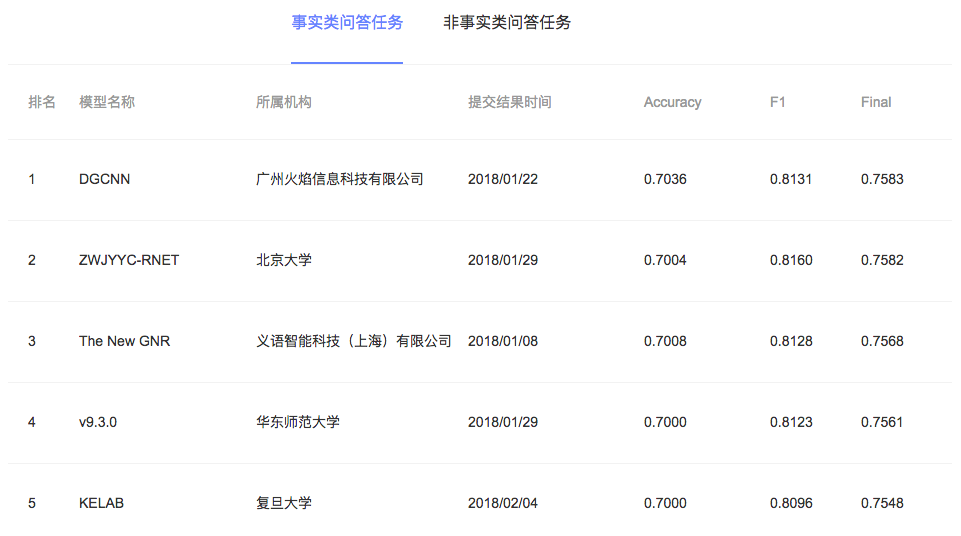
DGCNN stands for Dilated Gated Convolutional Neural Network. As the name suggests, it integrates two relatively new convolutional techniques: Dilated Convolution and Gated Convolution, while adding some manual features and tricks. This allows the model to achieve optimal results while remaining light and fast. At the time of writing, the model introduced here is at the top of the leaderboard with a score (average of accuracy and F1) of 0.7583. It is the only model so far that has never dropped out of the top three and has won the most weekly championships.
Competition Context
Actually, this model is a product of my participation in the CIPS-SOGOU Question Answering Competition on behalf of Guangzhou Flame Technology Co., Ltd. This competition started last October, but it has been somewhat anticlimactic, remaining in a state of limbo (no sign of ending, yet no new tasks).
In the first two or three months, the competition was quite intense. Many companies and universities submitted models, and the leaderboard was constantly refreshed. I feel SOGOU’s handling of the competition is a bit unfair to the initial enthusiasm of the participants. Most importantly, there have been no public notices regarding plans, changes, or the end date; contestants have simply been left waiting. I later heard the deadline is before this year’s CIPS... a competition lasting a whole year??
Task Description
So far, the SOGOU competition has only held the factoid portion, which is essentially the same as the WebQA dataset previously released by Baidu. It follows the format of "one question + multiple documents," with the goal of deciding the precise answer (usually an entity fragment) from the multiple documents.
Question: How many years of social security contributions are needed to receive a pension?
Answer: 15 years
Document 1: It’s best not to quit; if you pay for 15 years until retirement, you can receive a pension. If there are special reasons to quit, you can continue paying individually.
Document 2: Hello! If you have paid social security for 15 years and reach retirement age, you can receive a pension.
Document 3: In life, everyone pays social security. How many years until retirement... How many years do you need to pay social security to get a pension? The above text introduces this for everyone.
Compared to WebQA, the training set provided by Sogou has much more noise, which increases the difficulty of prediction. Furthermore, I believe this WebQA-style task leans towards retrieval matching and preliminary semantic understanding, which differs significantly from the SQuAD task (one long document + multiple questions). In SQuAD, some questions involve complex reasoning, which is why the top models on the SQuAD leaderboard are quite complex and massive.
Model
Now, let’s formally dive into the model introduction.
Architecture Overview
First, let’s look at the overall model diagram:
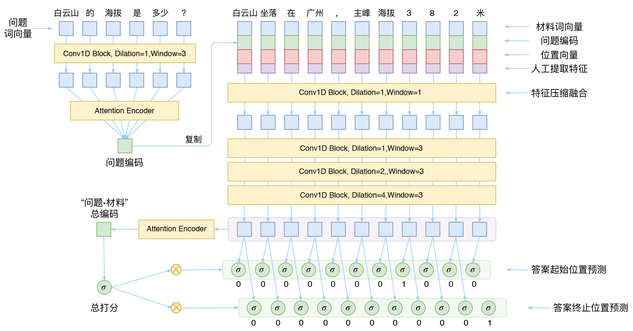
As seen in the diagram, for a "reading comprehension" or "QA system" model, the architecture is almost as simple as it gets.
The overall architecture is derived from the WebQA reference paper "Dataset and Neural Recurrent Sequence Labeling Model for Open-Domain Factoid Question". That paper has several characteristics:
It directly encodes the question using an LSTM to get a "question encoding," which is then concatenated to every word vector in the document.
It extracts two manual co-occurrence features.
It transforms the final prediction into a sequence labeling task solved with a CRF.
DGCNN basically follows this line of thought. Our differences are:
All LSTM parts in the original model are replaced with CNNs.
Richer co-occurrence features (8 in total) are extracted.
The CRF is removed and replaced with "0/1 labeling" to separately identify the start and end positions of the answer. This can be seen as a "half-pointer, half-labeling" structure.
Convolutional Structure
In this section, we analyze the Conv1D Block shown in the diagram.
Gating Mechanism
The convolutional structure used in the model comes from Facebook’s "Convolutional Sequence to Sequence Learning". Assuming the vector sequence we want to process is \boldsymbol{X}=[\boldsymbol{x}_1,\boldsymbol{x}_2,\dots,\boldsymbol{x}_n], we can add a gate to a standard 1D convolution: \boldsymbol{Y}=\text{Conv1D}_1(\boldsymbol{X}) \otimes \sigma\Big(\text{Conv1D}_2(\boldsymbol{X})\Big)\tag{1} Note that the two Conv1D operations have the same form (e.g., same number of filters and window size), but weights are not shared, meaning the parameters are doubled. One is activated with a sigmoid function, while the other has no activation function, and they are then multiplied element-wise. Since the range of the sigmoid function is (0,1), intuitively, it acts as a "valve" for each output of the Conv1D to control the flow. This is the GCNN structure, also known as a Gated Linear Unit (GLU).
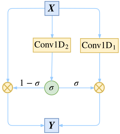
Besides its intuitive meaning, an advantage of using GCNN is the lower risk of vanishing gradients, as one part of the convolution does not have an activation function. If the input and output dimensions are the same, we add the input to the result, using a residual structure: \boldsymbol{Y}=\boldsymbol{X} + \text{Conv1D}_1(\boldsymbol{X}) \otimes \sigma\Big(\text{Conv1D}_2(\boldsymbol{X})\Big)\tag{2} It is worth mentioning that we use residual structures not just to solve vanishing gradients, but to allow information to flow through multiple channels. We can rewrite the above equation in a more illustrative equivalent form to see how information flows: \begin{aligned}\boldsymbol{Y}=&\boldsymbol{X}\otimes \Big(1-\boldsymbol{\sigma}\Big) + \text{Conv1D}_1(\boldsymbol{X}) \otimes \boldsymbol{\sigma}\\ \boldsymbol{\sigma} =& \sigma\Big(\text{Conv1D}_2(\boldsymbol{X})\Big) \end{aligned}\tag{3} From equation (3), we can see the flow more clearly: information passes through directly with probability 1-\sigma, and passes through after transformation with probability \sigma. This form is very similar to the GRU model in RNNs.
Supplementary Derivation: \begin{aligned}\boldsymbol{Y}=&\boldsymbol{X}\otimes \Big[1-\sigma\Big(\text{Conv1D}_2(\boldsymbol{X})\Big)\Big] + \text{Conv1D}_1(\boldsymbol{X}) \otimes \sigma\Big(\text{Conv1D}_2(\boldsymbol{X})\Big)\\ =&\boldsymbol{X} + \Big(\text{Conv1D}_1(\boldsymbol{X}) - \boldsymbol{X}\Big)\otimes \sigma\Big(\text{Conv1D}_2(\boldsymbol{X})\Big) \end{aligned} Since \text{Conv1D}_1 has no activation function, it is just a linear transformation. Thus, \text{Conv1D}_1(\boldsymbol{X}) - \boldsymbol{X} can be combined into a single \text{Conv1D}_1. Simply put, during training, whatever \text{Conv1D}_1(\boldsymbol{X}) - \boldsymbol{X} can achieve, \text{Conv1D}_1(\boldsymbol{X}) can also achieve. Thus, (2) and (3) are equivalent.
Dilated Convolution
Next, to allow the CNN model to capture longer distances without increasing model parameters, we use Dilated Convolution.
The comparison between standard convolution and dilated convolution can be demonstrated with a diagram:

Both are three-layer CNNs (the first layer is the input) with a window size of 3. In standard convolution, by the third layer, each node can only capture 3 inputs, remaining completely disconnected from other inputs.
In contrast, dilated convolution at the third layer can capture 7 inputs, but the number of parameters and speed remain unchanged. This is because, in the second layer, the dilated convolution skips inputs directly adjacent to the center and captures the center and the next-adjacent inputs (dilation rate of 2). This can be seen as a "window size of 5 with two holes." Thus, dilated convolution is also called Atrous Convolution. In the third layer, it skips three inputs (dilation rate of 4), which can be seen as a "window size of 9 with 6 holes." If you draw lines connecting related inputs and outputs, you will find that any node in the third layer is connected to 7 original inputs.
Following the principle of "avoiding overlap and omission as much as possible," the dilation rate usually grows geometrically: 1, 2, 4, 8, ... Of course, "as much as possible" is key, as there is still some overlap. This ratio is inspired by Google’s WaveNet model.
Block
Now we can explain the Conv1D Blocks in the model diagram. If the input and output dimensions are the same, it uses the dilated version of equation (3). If they differ, it uses the simple equation (1). Window sizes and dilation rates are noted in the diagram.
Attention
As seen in the model diagram, in the DGCNN model, Attention is primarily used to replace simple Pooling to integrate sequence information, including encoding the question vector sequence into a single question vector and the document sequence into a single document vector. The Attention used here is slightly different from the one in "Attention is All You Need". This can be considered a "Additive Attention" in the form: \begin{aligned}\boldsymbol{x}&=\text{Encoder}\big(\boldsymbol{x}_1,\boldsymbol{x}_2,\dots,\boldsymbol{x}_n\big)=\sum_{i=1}^n \lambda_i \boldsymbol{x}_i\\ \lambda_i&=\mathop{\text{softmax}}_i\Big(\boldsymbol{\alpha}^{\top}\,\text{Act}\big(\boldsymbol{W}\boldsymbol{x}_i\big)\Big)\end{aligned}\tag{4} Here \boldsymbol{\alpha}, \boldsymbol{W} are trainable parameters. \text{Act} is an activation function, usually \tanh, or potentially the \text{swish} function. When using \text{swish}, it is better to include bias terms: \lambda_i=\mathop{\text{softmax}}_i\Big(\boldsymbol{\alpha}^{\top}\,\text{Act}\big(\boldsymbol{W}\boldsymbol{x}_i+\boldsymbol{b}\big)+\beta\Big)\tag{5} This Attention scheme is referenced from the R-Net model. (Note: It might not have originated with R-Net, but that is where I learned it.)
Position Embedding
To enhance the CNN’s sense of position, we also add Position Embeddings, concatenated to each word vector in the document. The construction method follows the scheme in "Attention is All You Need": \left\{\begin{aligned}&PE_{2i}(p)=\sin\Big(p/10000^{2i/{d_{pos}}}\Big)\\ &PE_{2i+1}(p)=\cos\Big(p/10000^{2i/{d_{pos}}}\Big) \end{aligned}\right.\tag{6}
Output Design
This part is a unique feature of our model.
Logic Analysis
By now, the overall structure of the model should be clear. First, we encode the question into a fixed vector via convolution and attention. This vector is concatenated to every word vector in the document, along with position embeddings and manual features. At this point, we obtain a feature sequence mixed with question and document information. We process this sequence directly with several layers of convolution for encoding and then perform sequence labeling without further question interaction.
In SQuAD evaluations, the document definitely contains the answer, and the answer’s position is labeled. Thus, SQuAD models typically perform two softmax operations over the sequence to predict the start and end positions, often called a "Pointer Network." However, in our WebQA-style QA, the document might not contain the answer. Therefore, we do not use softmax; instead, we use sigmoid for the entire sequence. This allows for cases where there is no answer in the document, as well as cases where the answer appears multiple times.
Dual Labeling Output
Since we use labeling, the simplest theoretical scheme is to output a 0/1 sequence: directly labeling each word in the document as "is (1)" or "is not (0)" part of the answer. However, this doesn’t work well because an answer might consist of multiple consecutive words. Forcing the model to give the same label to different words might be "asking too much of the model." Thus, we still use two labeling tasks to separately label the start and end positions of the answer: \begin{aligned}p^{start}_i = \sigma\Big(\boldsymbol{\alpha}_1^{\top}\,\text{Act}\big(\boldsymbol{W}_1\boldsymbol{x}_i+\boldsymbol{b}_1\big)+\beta_1\Big)\\ p^{end}_i = \sigma\Big(\boldsymbol{\alpha}_2^{\top}\,\text{Act}\big(\boldsymbol{W}_2\boldsymbol{x}_i+\boldsymbol{b}_2\big)+\beta_2\Big)\end{aligned}\tag{7} In this way, the model’s output design is different from both the pointer method and pure sequence labeling, or rather, it is a simplification and fusion of both.
Global Perspective
Finally, to increase the model’s "big picture" view, we encode the document sequence into a single global vector, followed by a fully connected layer to get a global score. This score is multiplied by the previous labeling results: \begin{aligned}\boldsymbol{o}=&\text{Encoder}\big(\boldsymbol{x}_1,\boldsymbol{x}_2,\dots,\boldsymbol{x}_n\big)\\ p^{global}=&\sigma\Big(\boldsymbol{W}\boldsymbol{o}+\boldsymbol{b}\Big)\\ p^{start}_i =& p^{global}\cdot\sigma\Big(\boldsymbol{\alpha}_1^{\top}\,\text{Act}\big(\boldsymbol{W}_1\boldsymbol{x}_i+\boldsymbol{b}_1\big)+\beta_1\Big)\\ p^{end}_i =& p^{global}\cdot\sigma\Big(\boldsymbol{\alpha}_2^{\top}\,\text{Act}\big(\boldsymbol{W}_2\boldsymbol{x}_i+\boldsymbol{b}_2\big)+\beta_2\Big)\end{aligned}\tag{8} This global score is significant for model convergence and performance. Its role is to better judge whether an answer exists in the document. If no answer exists, the model can simply set p^{global}=0 without having to "painstakingly" force every word’s label to 0.
Handcrafted Features
We have mentioned manual features several times. How much do they help? By simple observation, these manual features might improve model performance by more than 2%! It is clear that well-designed features play a crucial role in improving performance and reducing model complexity.
Handcrafted features are designed for words in the document (Q for question, E for evidence/document).
Q-E Full Match
This checks if a word in the document appears in the question (1 if yes, 0 if no). The idea is to tell the model where question words appear in the document, as answers are likely to be near those locations. This aligns with how humans perform reading comprehension.
E-E Co-occurrence
This feature calculates the proportion of other documents in which a specific document word appears. For example, if there are 10 documents and a word w in the first document appears in 4 of the other nine documents, the word w in the first document gets a feature value of 4/10.
The logic is that the more documents a word appears in, the more likely it is to be the answer.
Q-E Soft Match
Using the question size as a window, we calculate Jaccard similarity and relative edit distance for each window in the document.
For example, if the question is "What is the altitude of Baiyun Mountain?" and the document is "Baiyun Mountain is located in Guangzhou, the main peak altitude is 3 8 2 meters." If the question has 6 words, the window size is 6. We split the document into windows and calculate the Jaccard similarity of each block with the question, using the result as a feature for the current word.
Similarly, we calculate the edit distance of each block with the question and divide it by the window size to get a value between 0 and 1, which I call "relative edit distance."
Jaccard similarity is order-independent, while edit distance is order-dependent. Thus, these two methods measure similarity from both unordered and ordered perspectives. The logic is the same as the first feature: telling the model which parts of the document are similar to the question.
The main idea for these two features came from Yin-shen in the Keras group. Thanks!
Character Features
Top models in SQuAD usually input both word and character vectors. To improve results, we should also input both. However, we didn’t want to make the model too massive, so we added character-level information via manual features.
The idea is simple: the four features mentioned above are calculated at the word level. We can also calculate them at the character level, then average the results of the characters within each word to serve as a word feature. For example, in the "Q-E Full Match," if the question contains the word "act" and the document contains "co-act," the word-level match is 0. But if we look at characters, "co-act" is split into "c", "o", "-", "a", "c", "t". Matching these against the characters in "act" gives 1 for "a", "c", "t" and 0 for the others. Averaging these gives 0.5 as the character-level "Q-E Full Match" feature for the word "co-act."
The other three features are handled similarly, giving us a total of 8 manual features.
Implementation
Now, all parts of the model have been explained. The overall model is simple and clear, giving a sense of "simplicity is beauty." Below are some implementation highlights.
Model Settings
Chinese Tokenization
As introduced, this model is word-based and incorporates character-level information through manual features. However, to make the model more flexible and able to answer more questions, I only performed basic tokenization to keep the granularity low.
Specifically: I wrote a unigram-based tokenization module with a dictionary of about 500,000 words. All English and numbers were split into individual letters and digits. For example, "apple" becomes five "words": a p p l e, and "382" becomes three "words": 3 8 2.
Since there is no new word discovery, the total vocabulary does not exceed 500,000. In fact, the final model has a vocabulary of only about 300,000.
Readers can use Jieba tokenization, disable new word discovery, and manually split numbers and English for the same effect.
Parameters
Word embedding dimension is 128, pre-trained using Word2Vec (Skip-Gram, window 5, 8 negative samples, 8 iterations) on the competition data, WebQA data, 500,000 Baidu Baike entries, and 1 million Baike Zhidao questions. Training took about 12 hours.
Padding uses zero vectors. Word embeddings are fixed during DGCNN training.
All Conv1D output dimensions are 128. Position embeddings are also 128.
Maximum sequence length is 100. Masking is applied to padding.
Since it’s a binary labeling task with class imbalance, binary Focal Loss is used as the loss function.
Trained with the Adam optimizer. First trained to optimum with a learning rate of 10^{-3} (about 6 epochs), then loaded the best model and trained with 10^{-4} (3 epochs).
Regularization
Late in the competition, we found a DropPath-like regularization slightly improved results.
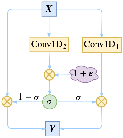
This regularization is built on equation (3). The idea is to perturb the "gate" during training: \begin{aligned}\boldsymbol{Y}=&\boldsymbol{X}\otimes \Big(1-\boldsymbol{\sigma}\Big) + \text{Conv1D}_1(\boldsymbol{X}) \otimes \boldsymbol{\sigma}\\ \boldsymbol{\sigma} =& \sigma\Big(\text{Conv1D}_2(\boldsymbol{X})\otimes (1 + \boldsymbol{\varepsilon})\Big) \end{aligned}\tag{9} where \boldsymbol{\varepsilon} is a uniform random noise tensor in [-0.1, 0.1]. This adds "multiplicative noise" to the GCNN gate to improve robustness against small parameter perturbations.
This scheme was inspired by regularization techniques in "FractalNet" and "Shake-Shake regularization."
Data Preparation
Preprocessing
Since the SOGOU competition allows external data, most teams used the WebQA dataset for supplementary training. Given that WebQA is relatively clean while SOGOU’s data is noisier, we mixed SOGOU and WebQA data in a 2:1 ratio.
Both datasets provide "one question + multiple documents + one answer" without specifying where the answer appears. Thus, we treated all substrings in the documents that matched the answer as answer locations. While this is occasionally unreasonable, it is the best approach without additional manual labeling.
There is also the issue of answer synonyms. For example, for the question "Who plays Mr. Bean?", the standard answer is "Rowan Atkinson," but documents might contain variations like "Rowan · Atkinson" or "Rowan . Atkinson." SOGOU provided an offline evaluation script that accounts for these variations, allowing us to identify and label synonymous answers.
Data Shuffling
SOGOU provided 30,000 labeled questions, pre-split into training (25,000) and validation (5,000). However, using this split resulted in validation performance that differed significantly from the online leaderboard.
We mixed all labeled data, shuffled it, and re-split it into training (20,000) and validation (10,000). This resulted in a validation score of about 0.76, close to the online results.
Data Augmentation
Three data augmentation operations were used:
Randomly zeroing out word IDs in the question and document: Since inputs are ID sequences (0 for padding/UNK), this randomly replaces words with UNK, reducing dependence on specific words.
Repeating and randomly cropping the same document to create new samples (the number and position of answers change accordingly).
For documents where the answer appears multiple times, randomly removing some answer labels.
The first method had the most significant impact on stability and accuracy. It differs from standard dropout on word vectors because it avoids scaling, making it more interpretable.
Decoding Strategy
A detail many contestants might overlook: The answer decoding method has huge room for optimization, and the improvement from optimizing decoding can be far greater than repeated hyperparameter tuning!
Scoring Method
What is answer decoding? Whether using softmax pointers or sigmoid labeling, the model outputs two columns of floats representing start and end scores. The question is: What metric determines the answer interval? The standard approach is to set a maximum answer length max_words (I used 10), then iterate through all intervals in the document within that length, calculating the sum or product of their start and end scores. Which is better: sum or product? Or the square root of the product?
Initially, I went with my gut and thought the square root of the product was most reasonable. Later, I tested the product directly and found a significant improvement (1%). I realized this decoding decision is a crucial hyperparameter.
Voting Method
If the same fragment appears multiple times in a document, should we sum, average, or take the maximum score? And how do we vote on answers from multiple documents?
Suppose there are 5 documents, and their answers and scores are (A, 0.7), (B, 0.2), (B, 0.2), (B, 0.2), (B, 0.2). Should we output A or B? Some say "many hands make light work," suggesting B because the sum of its scores (0.8) is greater than A’s (0.7).
I disagree. In real life, an expert is not simply the sum of many laymen. While there is strength in numbers, 1+1 is often less than 2. In the above distribution, we should prefer A because it is close to 1 and stands out.
Thus, our voting must reflect two points: 1. Strength in numbers; 2. 1+1 < 2. Summing and averaging fail here. The simplest solution is "sum of squares":
For the same document, if a fragment appears multiple times, take only the maximum score. A single document is like "one person"; there’s no need to stack their opinions.
After this, each document "elects" its own answer. Treat each document as an "expert" or "layman" with a score. Sum the squares of the scores for identical answers across documents: s_a = \sum_{i=1}^n s^2_{a,i} Squaring amplifies the weight of high-score samples.
In the competition, I used a slightly different formula: s_a = \frac{\sum\limits_{i=1}^n s^2_{a,i}}{1+\sum\limits_{i=1}^n s_{a,i}} This also uses the sum of squares idea but adds a penalty for small samples in the denominator. This formula is smoother than a direct sum of squares.
Model Ensemble
With the above steps, reaching 0.74–0.75 on the SOGOU test set is achievable. To reach the top score of 0.7583, model ensembling is required.
Ensembling includes single-model and multi-model ensembling. Single-model ensembling means training the same architecture multiple times with different seeds/splits and averaging the results. Multi-model ensembling involves ensembling different architectures. For simplicity, we only did single-model ensembling.
This was based on K-fold cross-validation. We split the labeled data into k parts, using each part as a validation set once (training from scratch each time).
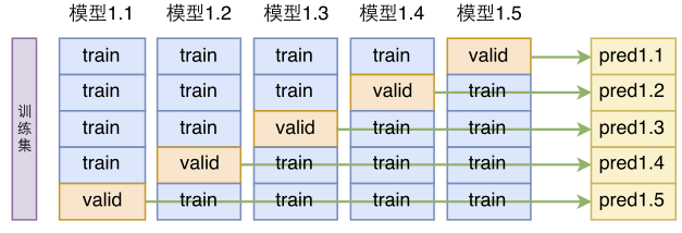
This gives k different training results for the same model, which are then averaged:
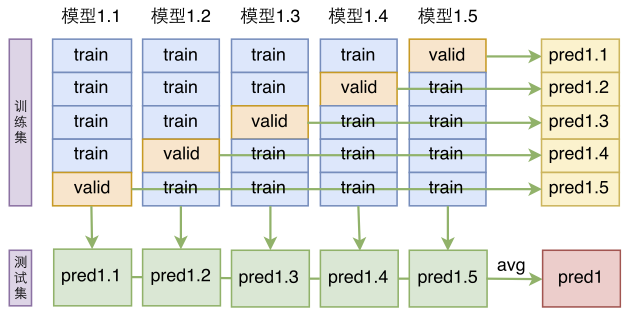
Conclusion
Effectiveness Evaluation
The leaderboard speaks for itself. On the noisy SOGOU test set, our model scored 0.7583. Looking at the training set, I suspect some noise was intentional; some documents were so irrelevant that a simple search engine recall wouldn’t be that bad. Therefore, I believe the effectiveness in actual use would be even better. Combined with the lightweight nature of a pure CNN, this fully meets industrial requirements.
Additionally, I tested this model on SQuAD and found the accuracy to be around 50% without fine-tuning or ensembling. With optimization, it might reach 60%+. This gap from 0.7583 shows that WebQA-style reading comprehension is very different from SQuAD’s pure reading comprehension, even if their models are theoretically interchangeable.
Code & Testing
The model is live on Flame Technology’s official website for online testing: http://www.birdbot.cn/online-factual-qa.html (Mobile access might be suboptimal; please use a PC.)
The code will not be made public for two reasons. First, I represented the company in this competition, so I cannot open-source everything. The model is simple enough that implementing it based on this article is not difficult. Second, once code is open-sourced, some readers skip the article and ask endless questions about environment setup or code errors.
This is not a "for dummies" post, so I ask for your understanding. This blog often has introductory articles, but this isn’t one of them. Furthermore, as a participant, I cannot directly release SOGOU’s training data. Readers can use the WebQA dataset for training.
Trial and Error
Finally, here is a screenshot:
This screenshot represents my entire debugging process, involving hundreds of iterations, with multiple experiments for each update. This is the most effort I’ve ever put into a competition.
So, while this is not a formal paper, if you have gained something from this article, I hope you will cite it.
Finally, thanks to Guangzhou Flame Technology for the software and hardware support and for providing me with excellent opportunities for growth.
PS: I later discovered that this model "collided" with the papers "Fast Reading Comprehension with ConvNets" and "QANET: Combining Local Convolution with Global Self-Attention for Reading Comprehension". However, I had never referenced those papers during the competition. I started from the WebQA paper, intended to reproduce it, tried a CNN model out of curiosity, and never looked back.
Original Link: https://kexue.fm/archives/5409