In the past, although I hadn’t looked into it closely, I always had the impression that Variational Autoencoders (VAE) were a good thing. Taking advantage of my recent short-lived enthusiasm for Probabilistic Graphical Models, I decided to try and understand VAE as well. As usual, I flipped through many online resources, and without exception, I found them quite vague. The main feeling was that while there were plenty of formulas, things remained blurry. Finally, when I thought I understood it and looked at the implementation code, I felt the code and the theory were not the same thing at all.
Finally, by piecing things together along with my accumulated knowledge of probabilistic models and repeatedly comparing with the original paper "Auto-Encoding Variational Bayes", I believe I have figured it out. In fact, the real VAE is quite different from what many tutorials describe. Many tutorials write a lot without capturing the key points of the model. Thus, I wrote this article, hoping to clarify VAE through the following text.
Distribution Transformation
We usually compare VAE with GAN. Indeed, their goals are basically consistent—both hope to construct a model that generates target data X from a latent variable Z. However, the implementations differ. More accurately, they assume that Z follows some common distribution (such as a normal or uniform distribution) and then hope to train a model X=g(Z) that can map the original probability distribution to the probability distribution of the training set. In other words, their purpose is to perform transformations between distributions.
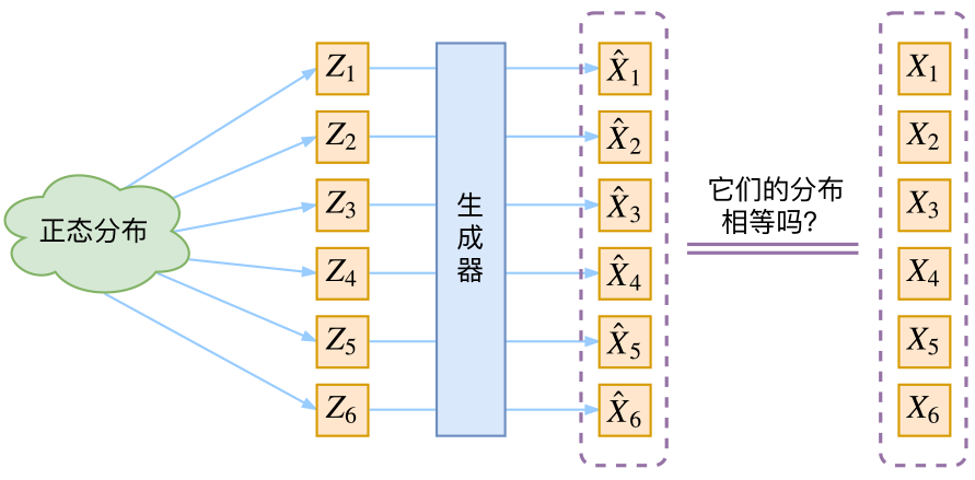
Now, suppose Z follows a standard normal distribution. I can sample several Z_1, Z_2, \dots, Z_n from it and transform them to get \hat{X}_1 = g(Z_1), \hat{X}_2 = g(Z_2), \dots, \hat{X}_n = g(Z_n). How do we judge whether the distribution of this dataset constructed through g is the same as our target dataset distribution? Some readers might suggest the KL divergence. Of course, that won’t work, because KL divergence is calculated based on the expressions of two probability distributions. However, we currently do not know the expressions of their probability distributions; we only have a batch of data \{\hat{X}_1, \hat{X}_2, \dots, \hat{X}_n\} sampled from the constructed distribution and a batch of data \{X_1, X_2, \dots, X_n\} sampled from the true distribution (the training set we wish to generate). We only have the samples themselves, no distribution expressions, and thus no way to calculate KL divergence.
Despite the difficulties, we must find a solution. GAN’s approach is direct and blunt: since there is no suitable metric, I will simply train that metric using a neural network. Thus, WGAN was born (for details, refer to "The Art of Mutual Confrontation: From Zero to WGAN-GP"). VAE, on the other hand, uses an exquisite and roundabout trick.
A Slow Talk on VAE
In this part, we first review how general tutorials introduce VAE, then explore what the problems are, and finally naturally discover the true face of VAE.
Classic Review
First, we have a batch of data samples \{X_1, \dots, X_n\}, described as X. We originally wanted to obtain the distribution p(X) from \{X_1, \dots, X_n\}. If we could get it, we could sample directly from p(X) to obtain all possible X (including those outside \{X_1, \dots, X_n\}). This would be an ultimate ideal generative model. Of course, this ideal is hard to achieve, so we modify the distribution: p(X)=\sum_Z p(X|Z)p(Z) \tag{1} Here we don’t distinguish between summation and integration; the meaning is what matters. At this point, p(X|Z) describes a model that generates X from Z, and we assume Z follows a standard normal distribution, i.e., p(Z)=\mathcal{N}(0,I). If this ideal could be realized, we could first sample a Z from the standard normal distribution and then calculate an X based on Z, which is also a great generative model. Next, this is combined with an autoencoder to implement reconstruction, ensuring no effective information is lost, followed by a series of derivations to implement the model. The schematic diagram of the framework is as follows:
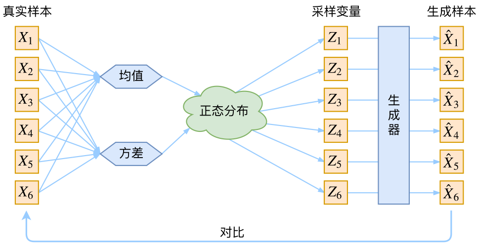
Do you see the problem? If it follows this diagram, we are actually not clear: does the resampled Z_k still correspond to the original X_k? Therefore, directly minimizing \mathcal{D}(\hat{X}_k, X_k)^2 (where \mathcal{D} represents some distance function) is unscientific. In fact, if you look at the code, you will find it is not implemented this way at all. In other words, many tutorials say a lot of things that sound reasonable, but when writing the code, they don’t follow their own words, yet they don’t seem to notice the contradiction.
The Emergence of VAE
In fact, in the entire VAE model, we do not use the assumption that p(Z) (the distribution of the latent variable space) is a normal distribution; we assume that p(Z|X) (the posterior distribution) is a normal distribution!!
Specifically, given a real sample X_k, we assume there exists an exclusive distribution p(Z|X_k) for X_k (technically called the posterior distribution), and further assume this distribution is a (independent, multivariate) normal distribution. Why emphasize "exclusive"? Because we later want to train a generator X=g(Z) and hope to reconstruct X_k from a Z_k sampled from the distribution p(Z|X_k). If we assumed p(Z) is a normal distribution and sampled a Z from p(Z), how would we know which real X this Z corresponds to? Now that p(Z|X_k) is exclusive to X_k, we have reason to say that a Z sampled from this distribution should be reconstructed back into X_k.
In fact, in the application part of the paper "Auto-Encoding Variational Bayes," this point is specifically emphasized:
In this case, we can let the variational approximate posterior be a multivariate Gaussian with a diagonal covariance structure: \log q_{\phi}(\boldsymbol{z}|\boldsymbol{x}^{(i)}) = \log \mathcal{N}(\boldsymbol{z} ;\boldsymbol{\mu}^{(i)},\boldsymbol{\sigma}^{2(i)}\boldsymbol{I}) \tag{9} (Note: This is directly quoted from the original paper; the symbols used in this article are not entirely consistent with the original paper, but I hope readers will not be confused.)
Equation (9) in the paper is the key to implementing the entire model. I don’t know why many tutorials fail to highlight it when introducing VAE. Although the paper also mentions that p(Z) is a standard normal distribution, that is not actually the most essential part.
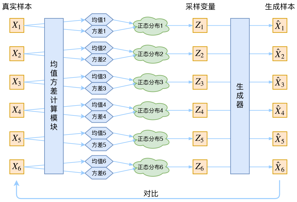
Returning to this article, each X_k is now paired with an exclusive normal distribution, facilitating the generator’s reconstruction. But this means there are as many normal distributions as there are X. We know a normal distribution has two sets of parameters: mean \mu and variance \sigma^2 (for multivariate cases, these are vectors). How do I find the mean and variance of the normal distribution p(Z|X_k) exclusive to X_k? There doesn’t seem to be a direct way. Well, I’ll use a neural network to fit them! This is the philosophy of the neural network era: if it’s hard to calculate, use a neural network to fit it. We already experienced this with WGAN, and now we experience it again.
So we construct two neural networks \mu_k = f_1(X_k) and \log \sigma_k^2 = f_2(X_k) to calculate them. We choose to fit \log \sigma_k^2 instead of \sigma_k^2 directly because \sigma_k^2 must be non-negative and requires an activation function, while \log \sigma_k^2 can be positive or negative and needs no activation. Now, I know the mean and variance exclusive to X_k, and thus I know what its normal distribution looks like. Then I sample a Z_k from this exclusive distribution and pass it through a generator to get \hat{X}_k=g(Z_k). Now we can safely minimize \mathcal{D}(\hat{X}_k, X_k)^2 because Z_k was sampled from the distribution exclusive to X_k; this generator should restore the original X_k. Thus, we can draw the schematic diagram of VAE:
Distribution Standardization
Let’s think about what results we will eventually get based on the training process shown above.
First, we want to reconstruct X, which means minimizing \mathcal{D}(\hat{X}_k, X_k)^2. However, this reconstruction process is affected by noise because Z_k is resampled, not directly calculated by the encoder. Obviously, noise increases the difficulty of reconstruction. Fortunately, the intensity of this noise (the variance) is calculated by a neural network. Therefore, to reconstruct better, the model will eventually try every means to make the variance zero. If the variance is zero, there is no randomness, so no matter how you sample, you get a deterministic result (the mean). Fitting one result is certainly easier than fitting many, and the mean is calculated by another neural network.
To put it bluntly, the model will slowly degenerate into a standard AutoEncoder, and the noise will no longer play a role.
Isn’t that a waste of effort? What about the promised generative model?
Don’t worry. In fact, VAE also forces all p(Z|X) to align with the standard normal distribution. This prevents the noise from becoming zero and ensures the model has generative capabilities. How to understand "ensuring generative capabilities"? If all p(Z|X) are very close to the standard normal distribution \mathcal{N}(0,I), then by definition: p(Z)=\sum_X p(Z|X)p(X)=\sum_X \mathcal{N}(0,I)p(X)=\mathcal{N}(0,I) \sum_X p(X) = \mathcal{N}(0,I) \tag{2} In this way, we can achieve our prior assumption: p(Z) is a standard normal distribution. Then we can safely sample from \mathcal{N}(0,I) to generate images.
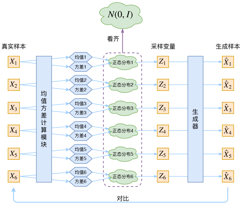
How do we make all p(Z|X) align with \mathcal{N}(0,I)? Without external knowledge, the most direct way is to add an extra loss to the reconstruction error: \mathcal{L}_{\mu}=\Vert f_1(X_k)\Vert^2 \quad \text{and} \quad \mathcal{L}_{\sigma^2}=\Vert f_2(X_k)\Vert^2 \tag{3} Because they represent the mean \mu_k and the logarithm of the variance \log\sigma_k^2, reaching \mathcal{N}(0,I) means hoping both are as close to 0 as possible. However, this faces the problem of how to choose the ratio between these two losses. If chosen poorly, the generated images will be blurry. Therefore, the original paper directly calculated the KL divergence between a general normal distribution (with independent components) and the standard normal distribution KL\Big(N(\mu,\sigma^2)\Big\Vert N(0,I)\Big) as this extra loss. The calculation result is: \mathcal{L}_{\mu,\sigma^2}=\frac{1}{2} \sum_{i=1}^d \Big(\mu_{(i)}^2 + \sigma_{(i)}^2 - \log \sigma_{(i)}^2 - 1\Big) \tag{4} where d is the dimension of the latent variable Z, and \mu_{(i)} and \sigma_{(i)}^2 represent the i-th components of the mean vector and variance vector of the general normal distribution. Using this formula as a supplementary loss avoids the need to consider the relative proportions of the mean loss and variance loss. Obviously, this loss can also be understood in two parts: \begin{aligned} &\mathcal{L}_{\mu,\sigma^2}=\mathcal{L}_{\mu} + \mathcal{L}_{\sigma^2}\\ &\mathcal{L}_{\mu}=\frac{1}{2} \sum_{i=1}^d \mu_{(i)}^2=\frac{1}{2}\Vert f_1(X)\Vert^2\\ &\mathcal{L}_{\sigma^2}=\frac{1}{2} \sum_{i=1}^d\Big(\sigma_{(i)}^2 - \log \sigma_{(i)}^2 - 1\Big) \end{aligned} \tag{5}
Derivation
Since we are considering a multivariate normal distribution with independent components, we only need to derive the case for a univariate normal distribution. According to the definition, we can write: \begin{aligned} &KL\Big(N(\mu,\sigma^2)\Big\Vert N(0,1)\Big)\\ =& \int \frac{1}{\sqrt{2\pi\sigma^2}}e^{-(x-\mu)^2/2\sigma^2} \left(\log \frac{e^{-(x-\mu)^2/2\sigma^2}/\sqrt{2\pi\sigma^2}}{e^{-x^2/2}/\sqrt{2\pi}}\right)dx\\ =& \int \frac{1}{\sqrt{2\pi\sigma^2}}e^{-(x-\mu)^2/2\sigma^2} \log \left\{\frac{1}{\sqrt{\sigma^2}}\exp\left\{\frac{1}{2}\big[x^2-(x-\mu)^2/\sigma^2\big]\right\} \right\}dx\\ =& \frac{1}{2}\int \frac{1}{\sqrt{2\pi\sigma^2}}e^{-(x-\mu)^2/2\sigma^2} \Big[-\log \sigma^2+x^2-(x-\mu)^2/\sigma^2 \Big] dx \end{aligned} The result is divided into three integral terms. The first term is actually -\log \sigma^2 multiplied by the integral of the probability density (which is 1), so the result is -\log \sigma^2. The second term is actually the second moment of the normal distribution; friends familiar with the normal distribution should know that the second moment is \mu^2+\sigma^2. According to the definition, the third term is actually "-variance divided by variance = -1". So the total result is: KL\Big(N(\mu,\sigma^2)\Big\Vert N(0,1)\Big)=\frac{1}{2}\Big(-\log \sigma^2+\mu^2+\sigma^2-1\Big)
Reparameterization Trick
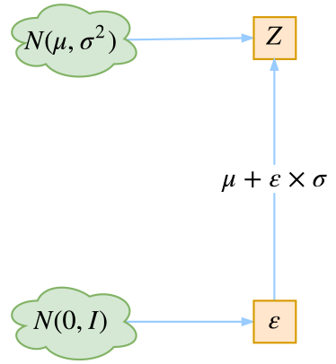
Finally, there is a trick for implementing the model, called the reparameterization trick. It’s actually very simple: we need to sample a Z_k from p(Z|X_k). Although we know p(Z|X_k) is a normal distribution, the mean and variance are calculated by the model. We need to optimize the mean and variance models through this process, but the "sampling" operation is non-differentiable, while the result of sampling is differentiable. We use: \begin{aligned} &\frac{1}{\sqrt{2\pi\sigma^2}}\exp\left(-\frac{(z-\mu)^2}{2\sigma^2}\right)dz \\ =& \frac{1}{\sqrt{2\pi}}\exp\left[-\frac{1}{2}\left(\frac{z-\mu}{\sigma}\right)^2\right]d\left(\frac{z-\mu}{\sigma}\right) \end{aligned} \tag{6} This shows that (z-\mu)/\sigma=\varepsilon follows a standard normal distribution with mean 0 and variance 1. We must consider dz because multiplying by dz makes it a probability; removing dz makes it a probability density, not a probability. At this point, we get:
Sampling a Z from \mathcal{N}(\mu,\sigma^2) is equivalent to sampling an \varepsilon from \mathcal{N}(0,I) and then letting Z=\mu + \varepsilon \times \sigma.
Thus, we change sampling from \mathcal{N}(\mu,\sigma^2) to sampling from \mathcal{N}(0,I), and then obtain the result of sampling from \mathcal{N}(\mu,\sigma^2) through parameter transformation. In this way, the "sampling" operation does not need to participate in gradient descent; instead, the result of the sampling does, making the entire model trainable.
As for the specific implementation, if you compare the above text with the code, you will understand it instantly.
Subsequent Analysis
Even after clarifying all the above content, we may still have many doubts about VAE.
What is the Essence?
What is the essence of VAE? Although VAE is called a type of AE (AutoEncoder), its approach (or its interpretation of the network) is unique. In VAE, there are two Encoders: one for calculating the mean and one for calculating the variance. This is already surprising: the Encoder is not used to Encode, but to calculate the mean and variance. This is big news. Also, aren’t mean and variance statistics? Why are they calculated by neural networks?
In fact, I think VAE starts from variational and Bayesian theories that are daunting to ordinary people and finally lands on a specific model. Although it takes a long path, the final model is actually very grounded: Essentially, it adds "Gaussian noise" to the output of the encoder (which corresponds to the network calculating the mean in VAE) on top of our conventional autoencoder, so that the decoder can be robust to noise; and that extra KL loss (aimed at making the mean 0 and variance 1) is actually equivalent to a regularization term for the encoder, hoping the encoder’s output has a zero mean.
What about the other encoder (corresponding to the network calculating the variance)? It is used to dynamically adjust the intensity of the noise. Intuitively, when the decoder is not yet well-trained (reconstruction error is much larger than KL loss), it will appropriately reduce the noise (KL loss increases), making fitting easier (reconstruction error starts to drop); conversely, if the decoder is trained well (reconstruction error is smaller than KL loss), the noise will increase (KL loss decreases), making fitting more difficult (reconstruction error starts to increase again). At this point, the decoder must find ways to improve its generative capability.
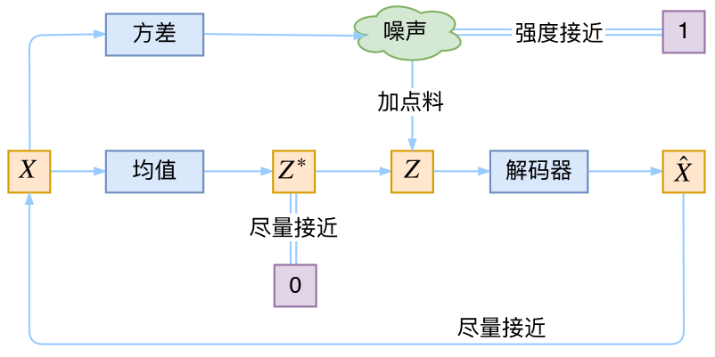
To put it simply, the reconstruction process hopes for no noise, while the KL loss hopes for Gaussian noise; the two are in opposition. Therefore, like GAN, VAE actually contains a process of confrontation internally, but the two are mixed together and evolve together. From this perspective, VAE’s idea seems even more sophisticated, because in GAN, when the counterfeiter evolves, the discriminator stays still, and vice versa. Of course, this is just one side; it doesn’t mean VAE is better than GAN. GAN’s true brilliance is that it even trains the metric directly, and this metric is often better than what we humans can think of (however, GAN itself has various problems, which won’t be expanded on here).
From this discussion, we can also see that each p(Z|X) cannot be exactly equal to the standard normal distribution; otherwise, p(Z|X) would be independent of X, and the reconstruction effect would be extremely poor. The final result will be that p(Z|X) retains some information about X, the reconstruction effect is acceptable, and equation (2) approximately holds, thus preserving generative capability.
Normal Distribution?
Regarding the distribution of p(Z|X), readers might wonder: is it necessary to choose a normal distribution? Can a uniform distribution be chosen?
It’s likely not feasible, mainly because of the KL divergence calculation formula: KL\Big(p(x)\Big\Vert q(x)\Big) = \int p(x) \ln \frac{p(x)}{q(x)}dx \tag{7} If p(x)\neq 0 and q(x)=0 in some region, the KL divergence becomes infinite. For a normal distribution, the probability density at all points is non-negative, so this problem does not exist. But for a uniform distribution, as long as the two distributions are inconsistent, there will inevitably be intervals where p(x)\neq 0 and q(x)=0, so the KL divergence will be infinite. Of course, when writing code, we prevent such division-by-zero errors, but we still cannot avoid the KL loss taking up a large proportion. Therefore, the model will rapidly reduce the KL loss, meaning the posterior distribution p(Z|X) rapidly tends toward the prior distribution p(Z), and the noise and reconstruction cannot play an adversarial role. This goes back to what we said at the beginning: it becomes impossible to distinguish which z corresponds to which x.
Of course, it’s not impossible to use a uniform distribution, but you’d have to calculate the KL divergence between two uniform distributions, handle division-by-zero errors, increase the weight of the reconstruction loss, etc. But that would look too ugly.
Where is the Variation?
Another interesting (but not very important) question is: VAE is called a "Variational Autoencoder"; what is its connection to the calculus of variations? In the VAE paper and related interpretations, there doesn’t seem to be any sign of the calculus of variations?
Well, if the reader has already accepted the KL divergence, then VAE really doesn’t seem to have much to do with variations. Theoretically, for the KL divergence (7), we need to prove:
Given a fixed probability distribution p(x) (or q(x)), for any probability distribution q(x) (or p(x)), KL\Big(p(x)\Big\Vert q(x)\Big)\geq 0 always holds, and it equals zero only when p(x)=q(x).
Because KL\Big(p(x)\Big\Vert q(x)\Big) is actually a functional, finding the extremum of a functional requires the calculus of variations. Of course, the calculus of variations here is just a parallel generalization of ordinary calculus and hasn’t involved truly complex variational methods. The variational lower bound of VAE is obtained directly based on KL divergence. So if you directly accept KL divergence, there’s no business for variations.
In short, the word "Variational" in VAE’s name is because its derivation process uses KL divergence and its properties.
Conditional VAE
Finally, since the current VAE is trained unsupervised, it’s natural to think: if there is labeled data, can we add label information to assist in generating samples? The intention of this question is often to hope to control a certain variable to generate a certain class of images. Of course, this is certainly possible; we call this situation Conditional VAE, or CVAE. (Correspondingly, in GAN, we have CGAN.)
However, CVAE is not a specific model but a class of models. In short, there are many ways to integrate label information into VAE, and the purposes vary. Based on the previous discussion, here is a very simple CVAE.
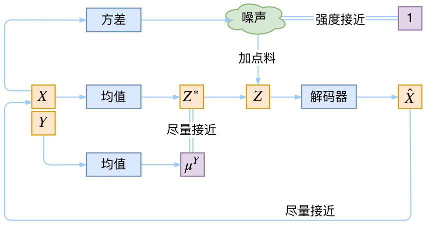
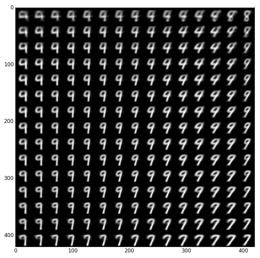
In the previous discussion, we hoped that after X is encoded, the distribution of Z would have zero mean and unit variance. This "hope" was achieved by adding KL loss. If we now have category information Y, we can hope that samples of the same class have an exclusive mean \mu^Y (variance remains unchanged, still unit variance), and let the model train this \mu^Y itself. In this way, there are as many normal distributions as there are classes, and during generation, we can control the category of the generated image by controlling the mean. In fact, this might be the scheme that adds the least code to VAE to implement CVAE, because this "new hope" only needs to be implemented by modifying the KL loss: \mathcal{L}_{\mu,\sigma^2}=\frac{1}{2} \sum_{i=1}^d\Big[\big(\mu_{(i)}-\mu^Y_{(i)}\big)^2 + \sigma_{(i)}^2 - \log \sigma_{(i)}^2 - 1\Big] \tag{8} The figure below shows that this simple CVAE has some effect, but because the encoder and decoder are relatively simple (pure MLP), the control effect is not perfect. For a more complete CVAE, readers should study on their own. Recently, work combining CVAE and GAN has also emerged, such as CVAE-GAN; model strategies are ever-changing.
Code
I copied the official Keras VAE code, fine-tuned it, added Chinese comments based on the previous content, and also implemented the simple CVAE mentioned at the end for readers’ reference.
The Final Stop
After some bumps, we have reached the end of the article. I don’t know if I’ve made it clear; I hope everyone will provide more feedback.
Overall, the idea of VAE is very beautiful. It’s not so much that it provides a great generative model (because in fact, the images it generates are not that good and tend to be blurry), but rather that it provides a very good case of combining probability graphs with deep learning. This case has many places worth thinking about and savoring.
When reprinting, please include the original address of this article: https://kexue.fm/archives/5253
For more detailed reprinting matters, please refer to: "Scientific Space FAQ"