In fact, shortly after the paper Dynamic Routing Between Capsules was released, a new Capsule paper titled Matrix Capsules with EM Routing was made public anonymously (during the ICLR 2018 anonymous review process). Now that the authors have been revealed, they are indeed Geoffrey Hinton, Sara Sabour, and Nicholas Frosst. As expected, Hinton is among them.
As everyone knows, results published by "pioneer-level" figures like Hinton are generally quite "heavyweight." So, what are the characteristics of this new paper?
During my thinking process, the article Understanding Matrix capsules with EM Routing provided me with much inspiration, and discussions by various experts on Zhihu also accelerated my reading. I would like to express my gratitude here.
Abstract
Let us first recall the diagram from the previous introduction Another New Year’s Eve Feast: From K-Means to Capsule:
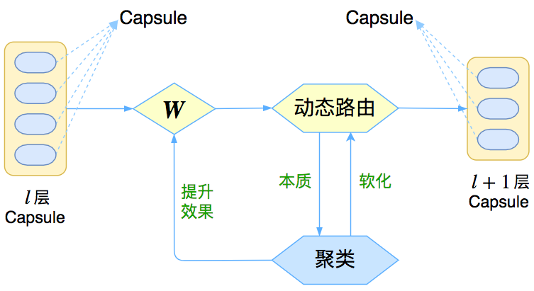
This diagram indicates that Capsule actually describes a modeling framework where many components can be customized. The most obvious one is the clustering algorithm; one could say, "There are as many types of dynamic routing as there are clustering algorithms." So, what did Hinton modify this time? Overall, this new paper introduces the following new elements:
Previously, a Capsule was represented by a vector; now it is represented by a matrix.
The clustering algorithm has been replaced with GMM (Gaussian Mixture Model).
In the experimental section, a Capsule version of convolution is implemented.
A Wave of Questions
In fact, seeing these three new things I proposed, readers might have many thoughts and questions, such as:
Vector vs. Matrix
What is the difference between a matrix and a vector? Can’t a matrix be flattened into a vector?
There is actually a slight difference. For example, what is the difference between a 4 \times 4 matrix and a 16-dimensional vector? The answer is that the importance of elements at different positions in a matrix varies, whereas in a vector, every element’s importance is treated the same. Readers familiar with linear algebra might also feel that the diagonal elements of a matrix "seem" more important than others. From a computational perspective, to transform a 16-dimensional vector into another 16-dimensional vector, we need a 16 \times 16 transformation matrix; however, to transform a 4 \times 4 matrix into another 4 \times 4 matrix, we only need a 4 \times 4 transformation matrix, which reduces the number of parameters. From this perspective, the fundamental purpose of changing Capsules from vectors to matrices might be to reduce the computational load.
Cubic Arrays?
Could future Capsules be "cubic arrays" or even higher-order tensors?
Unlikely. This is because the multiplication of higher-order tensors is essentially the multiplication of second-order matrices.
GMM vs. K-Means
Is GMM clustering very different from the K-Means clustering mentioned before?
This must be viewed from two perspectives. On one hand, GMM can be seen as an upgraded version of K-Means, and it is inherently differentiable, requiring no "softening" tricks. If Euclidean distance is used in K-Means, then K-Means is a limiting version of GMM. On the other hand, K-Means allows us to use other similarity measures more flexibly, while GMM essentially restricts us to (weighted) Euclidean distance, which "hardcodes" the metric. This can be considered a disadvantage. Overall, they are roughly equal in merit.
Capsule Convolution
What is the Capsule version of convolution? Why wasn’t it in the previous paper?
The dynamic routing we speak of is essentially equivalent to a fully connected layer in deep learning, while a convolutional layer is a local fully connected layer. Thus, by simply creating "local dynamic routing," we obtain the Capsule version of convolution. This should have appeared in Hinton’s previous paper, as it is independent of the specific routing algorithm, but for some reason, Hinton only implemented it in this new paper.
Introduction to the GMM Model
Since this new paper uses GMM for clustering, we must spend some effort learning about GMM. Understanding the GMM algorithm is very interesting, even if not for the sake of Capsules, because the GMM model greatly deepens our understanding of probabilistic models and machine learning theory (especially unsupervised learning theory). As a preview, in the following content, I have significantly simplified the derivation process of GMM, which I believe will reduce the difficulty of understanding.
Of course, readers who only want to understand the core idea of Capsules can selectively skip the more theoretical parts.
Essence
In fact, it is best not to view GMM merely as a clustering algorithm, but as a true unsupervised learning algorithm that attempts to learn the distribution of data. Data points are individuals, while the distribution is a whole. Moving from studying data itself to studying the data distribution is a qualitative change.
GMM stands for Gaussian Mixture Model. Specifically, for existing vectors \mathbf{x}_1, \dots, \mathbf{x}_n, GMM hopes to find the distribution p(\mathbf{x}) they satisfy. Of course, we cannot search aimlessly; we need a relatively simple form. GMM assumes that this batch of data can be divided into several parts (categories), each studied separately: p(\mathbf{x}) = \sum_{j=1}^k p(j)p(\mathbf{x}|j) \tag{1} where j represents the category, taking values 1, 2, \dots, k. Since p(j) is independent of \mathbf{x}, it can be considered a constant distribution, denoted as p(j) = \pi_j. Then p(\mathbf{x}|j) is the probability distribution within that category. The characteristic of GMM is using a probability distribution to describe a category. What should we choose for it? We take the simplest normal distribution. Note that \mathbf{x} is a vector, so we consider a multivariate normal distribution, generally in the form: N(\mathbf{x}; \boldsymbol{\mu}_j, \boldsymbol{\Sigma}_j) = \frac{1}{(2\pi)^{d/2}(\det\boldsymbol{\Sigma}_j)^{1/2}} \exp\left(-\frac{1}{2}(\mathbf{x}-\boldsymbol{\mu}_j)^{\top}\boldsymbol{\Sigma}_j^{-1}(\mathbf{x}-\boldsymbol{\mu}_j)\right) \tag{2} where d is the number of components in vector \mathbf{x}. Now we have the basic form of the model: p(\mathbf{x}) = \sum_{j=1}^k p(j) \times p(\mathbf{x}|j) = \sum_{j=1}^k \pi_j N(\mathbf{x}; \boldsymbol{\mu}_j, \boldsymbol{\Sigma}_j) \tag{3}
Solving the Model
Now that we have the model, the unknown parameters are \pi_j, \boldsymbol{\mu}_j, \boldsymbol{\Sigma}_j. How do we determine them?
The ideal method is Maximum Likelihood Estimation (MLE); however, it has no analytical solution and thus needs to be transformed into an EM process. Even then, the solving process is difficult to understand (involving derivatives of determinants). Here, I provide a simple and clear derivation based on the fact that for a normal distribution, the MLE results are the same as the results of the method of moments for the first two moments. (Trust me, this should be one of the simplest GMM derivations you can find.)
Simply put, aren’t \boldsymbol{\mu}_j and \boldsymbol{\Sigma}_j just the mean (vector) and (co)variance (matrix) of the normal distribution? Can’t I just calculate the corresponding mean and variance directly from the samples? It’s not that simple, because we assumed a mixture model. If we calculate them directly, we only get the mixture mean and variance, not the mean and variance of each individual category p(\mathbf{x}|j).
However, we can use Bayes’ theorem to transform it. First, we have: p(j|\mathbf{x}) = \frac{p(\mathbf{x}|j)p(j)}{p(\mathbf{x})} = \frac{\pi_j N(\mathbf{x}; \boldsymbol{\mu}_j, \boldsymbol{\Sigma}_j)}{\sum_{j=1}^k \pi_j N(\mathbf{x}; \boldsymbol{\mu}_j, \boldsymbol{\Sigma}_j)} \tag{4}
For the mean vector, we have: \boldsymbol{\mu}_j = \int p(\mathbf{x}|j)\mathbf{x}d\mathbf{x} = \int p(\mathbf{x}) \frac{p(j|\mathbf{x})}{p(j)}\mathbf{x}d\mathbf{x} = E\left[\frac{p(j|X)}{p(j)}X\right] \tag{5} Here E[] denotes the mathematical expectation over all samples, so we get: \boldsymbol{\mu}_j = \frac{1}{n}\sum_{i=1}^n \frac{p(j|\mathbf{x}_i)}{p(j)}\mathbf{x}_i = \frac{1}{\pi_j n}\sum_{i=1}^n p(j|\mathbf{x}_i)\mathbf{x}_i \tag{6} where the expression for p(j|\mathbf{x}) is given in (4). Similarly, for the covariance matrix: \boldsymbol{\Sigma}_j = \frac{1}{\pi_j n}\sum_{i=1}^n p(j|\mathbf{x}_i)(\mathbf{x}_i-\boldsymbol{\mu}_j)(\mathbf{x}_i-\boldsymbol{\mu}_j)^{\top} \tag{7} And: \pi_j = p(j) = \int p(j|\mathbf{x})p(\mathbf{x})d\mathbf{x} = E\left[p(j|X)\right] \tag{8} So: \pi_j = \frac{1}{n}\sum_{i=1}^n p(j|\mathbf{x}_i) \tag{9}
Theoretically, we need to solve a massive system of equations formed by (4), (6), (7), and (9), but this is difficult to operate. Therefore, we can solve iteratively, obtaining the iteration algorithm:
EM Algorithm 1: \left\{\begin{aligned} &p(j|\mathbf{x}_i) \leftarrow \frac{\pi_j N(\mathbf{x}_i;\boldsymbol{\mu}_j,\boldsymbol{\Sigma}_j)}{\sum_{j=1}^k\pi_j N(\mathbf{x}_i;\boldsymbol{\mu}_j,\boldsymbol{\Sigma}_j)}\\ &\boldsymbol{\mu}_j \leftarrow \frac{1}{\sum_{i=1}^n p(j|\mathbf{x}_i)}\sum_{i=1}^n p(j|\mathbf{x}_i)\mathbf{x}_i\\ &\boldsymbol{\Sigma}_j \leftarrow \frac{1}{\sum_{i=1}^n p(j|\mathbf{x}_i)}\sum_{i=1}^n p(j|\mathbf{x}_i)(\mathbf{x}_i-\boldsymbol{\mu}_j)(\mathbf{x}_i-\boldsymbol{\mu}_j)^{\top}\\ &\pi_j \leftarrow \frac{1}{n}\sum_{i=1}^n p(j|\mathbf{x}_i) \end{aligned}\right.
To highlight the characteristics of weighted averaging, the above iteration process first performs an identity transformation on (9) and then substitutes it into (6) and (7). In the above iteration process, the first equation is called the E-step, and the latter three are called the M-step. The entire algorithm is called the EM algorithm. Below is an animation found online showing the GMM iteration process. It can be seen that the advantage of GMM is its ability to identify clusters of general quadratic surface shapes, whereas K-Means can only identify spherical ones.
[Click to view GIF: GMM Iteration Process]
![[Click to view GIF: GMM Iteration Process]](https://kexue.fm/usr/uploads/2018/02/3750634145.gif)
Reduction
In Capsules, a simpler form of GMM is actually used. In the previous discussion, we used a general normal distribution (Eq. 2), but this requires calculating matrix inverses and determinants, which is computationally expensive. A simpler model assumes the covariance matrix is a diagonal matrix \boldsymbol{\Sigma}_j = \text{diag}(\boldsymbol{\sigma}^2_j), where \boldsymbol{\sigma}^2_j is the variance vector of category j. Thus \boldsymbol{\sigma}_j is the standard deviation vector, and \sigma_j^l represents the l-th component of that vector. This is equivalent to decoupling the components of \mathbf{x}, assuming they are independent. Eq. (2) then becomes: N(\mathbf{x};\boldsymbol{\mu}_j,\boldsymbol{\sigma}^2_j) = \prod_{l=1}^d \frac{1}{\sqrt{2\pi}\sigma_j^l} \exp\left(-\frac{1}{2(\sigma_j^l)^2}(x^l-\mu_j^l)^2\right) \tag{10} The iteration process is also simplified:
EM Algorithm 2: \left\{\begin{aligned} &p(j|\mathbf{x}_i) \leftarrow \frac{\pi_j N(\mathbf{x}_i;\boldsymbol{\mu}_j,\boldsymbol{\sigma}^2_j)}{\sum_{j=1}^k\pi_j N(\mathbf{x}_i;\boldsymbol{\mu}_j,\boldsymbol{\sigma}^2_j)}\\ &\boldsymbol{\mu}_j \leftarrow \frac{1}{\sum_{i=1}^n p(j|\mathbf{x}_i)}\sum_{i=1}^n p(j|\mathbf{x}_i)\mathbf{x}_i\\ &\boldsymbol{\sigma}^2_j \leftarrow \frac{1}{\sum_{i=1}^n p(j|\mathbf{x}_i)}\sum_{i=1}^n p(j|\mathbf{x}_i)(\mathbf{x}_i-\boldsymbol{\mu}_j)^2 \quad [\text{element-wise square}]\\ &\pi_j \leftarrow \frac{1}{n}\sum_{i=1}^n p(j|\mathbf{x}_i) \end{aligned}\right.
Even Simpler
If all \sigma_j^l are set to the same constant \sigma, we get: N(\mathbf{x};\boldsymbol{\mu}_j,\sigma) = \frac{1}{\sqrt{2\pi}\sigma^d} \exp\left(-\frac{1}{2\sigma^2}\Vert \mathbf{x}-\boldsymbol{\mu}_j\Vert^2\right) \tag{11} This makes the entire distribution even simpler. Interestingly, Euclidean distance appears within the exponent.
More extremely, if we let \sigma \to 0, the term in the exponent becomes negative infinity. It is not hard to prove that for each \mathbf{x}_i, only the N(\mathbf{x}_i;\boldsymbol{\mu}_j,\sigma^2) that minimizes \Vert \mathbf{x}_i-\boldsymbol{\mu}_j\Vert^2 dominates. At this point, according to Eq. (4), p(j|\mathbf{x}_i) is either 0 or 1. This indicates that any point belongs only to the nearest cluster center, which is consistent with K-Means using Euclidean distance. Thus, K-Means based on Euclidean distance can be seen as a limit of GMM.
The New Version of Routing
Returning to the main topic: Capsules. We said that Matrix Capsules with EM Routing uses the GMM algorithm to complete the clustering process. Let’s look at how it’s done in detail.
Matrix \to Vector
It must be said that the notation in the new paper is a mess. Perhaps being able to see the truth amidst a pile of chaotic symbols is what makes one a true expert. Here, combining some popular science materials and my own reading, I provide some interpretations.
First, we use a matrix \mathbf{P}_i to represent the Capsules in layer l. There are n Capsules in this layer, so i=1, \dots, n. We use matrix \mathbf{M}_j to represent the Capsules in layer l+1. There are k Capsules in this layer, meaning they are clustered into k categories, j=1, \dots, k. The Capsule matrices in the paper are 4 \times 4, called Pose matrices. Then, the GMM process begins. During GMM, the matrices are treated as vectors, so in EM routing, \mathbf{P}_i is a vector with d=16. The entire process uses a simplified version of GMM, where the covariance matrix is assumed to be diagonal.
Based on our previous discussion, we obtain the new dynamic routing algorithm:
New Dynamic Routing 1: \left\{\begin{aligned} &p_{ij} \leftarrow N(\mathbf{P}_i;\boldsymbol{\mu}_j,\boldsymbol{\sigma}^2_j)\\ &R_{ij} \leftarrow \frac{\pi_j p_{ij} }{\sum_{j=1}^k\pi_j p_{ij} }, \quad r_{ij} \leftarrow \frac{R_{ij}}{\sum_{i=1}^n R_{ij}}\\ &\mathbf{M}_j \leftarrow \sum_{i=1}^n r_{ij}\mathbf{P}_i\\ &\boldsymbol{\sigma}^2_j \leftarrow \sum_{i=1}^n r_{ij}(\mathbf{P}_i-\mathbf{M}_j)^2\\ &\pi_j \leftarrow \frac{1}{n}\sum_{i=1}^n R_{ij} \end{aligned}\right. Here we denote p_{ij}=N(\mathbf{x}_i;\boldsymbol{\mu}_j,\boldsymbol{\sigma}^2_j) and R_{ij}=p(j|\mathbf{x}_i). The notation is kept as consistent as possible with the original paper for comparison. The idea of dynamic routing here is consistent with Dynamic Routing Between Capsules: treating layer l+1 Capsules as the cluster centers of layer l Capsules, just with a different clustering method.
Activation Values
In the paper Dynamic Routing Between Capsules, the length of the vector represents the significance of the feature. Can we still do this here? The answer is no. Because we use GMM for clustering, which is based on weighted Euclidean distance, a characteristic of Euclidean clustering is that the cluster center vector is the (weighted) average of the vectors in the cluster (as seen from the iteration formula for \mathbf{M}_j). Since it is an average, it cannot reflect the "more followers, more power" characteristic, as mentioned in Another New Year’s Eve Feast: From K-Means to Capsule.
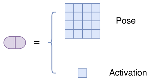
Since the length of the Capsule can no longer measure feature significance, we must add a scalar a to represent the Capsule’s significance. Thus, a Capsule in this paper is actually "a matrix + a scalar." This scalar is called the "activation value," as shown:
As the significance of a Capsule, the most direct choice for a_j should be \pi_j, because the layer l+1 Capsule is the cluster center and \pi_j represents the probability of this category. However, we cannot choose \pi_j for two reasons:
\pi_j is normalized, but we want the significance of the feature itself, not its relative significance compared to other features (more simply, we want to perform multiple binary classifications, not one multi-class classification, so global normalization is not needed).
While \pi_j reflects the number of "followers" in the category, a large number of followers doesn’t necessarily mean strength; they must also be united.
So how should this activation value be determined? The formula given in the paper is: a_j = \text{logistic}\left(\lambda\left(\beta_a - \beta_u \sum_i R_{ij} - \sum_h \text{cost}_j^h\right)\right) \tag{12} I believe many readers will still be confused after seeing this formula and the "derivation" in the paper. In fact, this formula has a very beautiful origin: information entropy.
Now that we use GMM for clustering, the result is a probability distribution p(\mathbf{X}|j) describing a category. The "degree of uncertainty" of this category can measure its "degree of cohesion." To put it more bluntly, the greater the "uncertainty" (meaning it’s closer to a uniform distribution), the more it suggests the category is in a state of turmoil or fragmentation, and the activation value should be smaller. The smaller the "uncertainty" (meaning the distribution is more concentrated), the more it suggests the category is united and modernized, and the activation value should be larger.
Therefore, uncertainty can describe this activation value. We know that uncertainty is measured by information entropy, so we write: \begin{aligned} S_j &= - \int p(\mathbf{x}|j)\ln p(\mathbf{x}|j)d\mathbf{x}\\ &= - \frac{1}{p(j)}\int p(j|\mathbf{x})p(\mathbf{x})\ln p(\mathbf{x}|j)d\mathbf{x}\\ &= - \frac{1}{p(j)} E\left[p(j|\mathbf{x})\ln p(\mathbf{x}|j)\right]\\ &= -\frac{1}{n\pi_j}\sum_{i=1}^n R_{ij}\ln p_{ij}\\ &= -\frac{1}{\sum_{i=1}^n R_{ij}}\sum_{i=1}^n R_{ij}\ln p_{ij}\\ &= -\sum_{i=1}^n r_{ij}\ln p_{ij} \end{aligned} \tag{13} This is the \text{cost}_j^h in the paper. So the "cost" in the paper is entropy—what a clear and intuitive meaning! And smaller entropy is better—what a natural logic! (Why not calculate the entropy of the normal distribution directly by integration instead of this roundabout way? Because integration gives a theoretical result; here we want to calculate an actual result based on the data batch itself.)
Note: If readers do not understand sampling calculation well, please read the section "Numerical Calculation vs. Sampling Calculation" in Variational Autoencoders (2): From a Bayesian Perspective.
After simplification, the result is (the calculation in the original paper seems to be incorrect): S_j = \frac{d}{2} + \left(\sum_{l=1}^d \ln \sigma_j^l + \frac{d}{2}\ln (2\pi)\right)\sum_i r_{ij} \tag{14}
Supplementary Derivation: The assumption here is that p_{ij} corresponds to a d-dimensional independent normal distribution, so we only need to find the entropy of each dimension and sum them: \begin{aligned} S_j^l &= \sum_{i} - r_{ij} \ln p_{ij}^l\\ &= \sum_{i} - r_{ij} \ln \left[\frac{1}{\sqrt{2\pi}\sigma_j^l}\exp\left(-\frac{(x_i^l-\mu_j^l)^2}{2(\sigma_j^l)^2}\right)\right]\\ &= \left(\frac{1}{2}\ln 2\pi + \ln\sigma_j^l\right)\sum_{i} r_{ij} + \frac{\sum_{i}r_{ij}(x_i^l-\mu_j^l)^2}{2(\sigma_j^l)^2} \end{aligned} Note that the numerator of the last term is actually the formula for calculating variance, and the denominator is twice the variance. So the last term is "variance/variance" divided by 2, which is 1/2. S_j^l = \sum_{i} - r_{ij} \ln p_{ij}^l = \left(\frac{1}{2}\ln 2\pi + \ln\sigma_j^l\right)\sum_{i} r_{ij} + \frac{1}{2} Thus: S_j = \sum_{l=1}^d S_j^l = \left(\frac{d}{2}\ln 2\pi + \sum_{l=1}^d\ln\sigma_j^l\right)\sum_{i} r_{ij} + \frac{d}{2}
Since smaller entropy means more significance, we use -S_j to measure feature significance, but we want to compress it between 0 and 1. We can perform a simple scale transformation and then use the sigmoid function: a_j = \text{sigmoid}\left( \lambda \left( \beta_a - \left(\beta_u + \sum_{l=1}^d \ln \sigma_j^l \right)\sum_i r_{ij}\right)\right) \tag{15} Eq. (15) and Eq. (13) are basically equivalent. The above equation is essentially a weighted sum of -S_j and \pi_j, considering both -S_j (unity) and \pi_j (numbers). \beta_a and \beta_u are optimized through backpropagation, while \lambda increases slowly during training (an annealing strategy chosen by the paper, which I think is unnecessary). \beta_a and \beta_u might depend on j, meaning a set of training parameters \beta_a, \beta_u can be assigned to each upper-layer capsule. I say "might" because the paper doesn’t explain it clearly; perhaps readers can adjust according to their own experiments and needs.
Routing Revealed
With the formula for a_j, and since we said a_j and \pi_j share commonalities as weights for the category, Hinton simply replaces \pi_j with a_j to make the routing process more compact. Although this replacement doesn’t perfectly correspond to the original GMM iteration, the meaning is similar and it converges. We now have the corrected dynamic routing:
New Dynamic Routing 2: \left\{\begin{aligned} &p_{ij} \leftarrow N(\mathbf{P}_i;\boldsymbol{\mu}_j,\boldsymbol{\sigma}^2_j)\\ &R_{ij} \leftarrow \frac{a_j p_{ij} }{\sum_{j=1}^k a_j p_{ij} }, \quad r_{ij} \leftarrow \frac{R_{ij}}{\sum_{i=1}^n R_{ij}}\\ &\mathbf{M}_j \leftarrow \sum_{i=1}^n r_{ij}\mathbf{P}_i\\ &\boldsymbol{\sigma}^2_j \leftarrow \sum_{i=1}^n r_{ij}(\mathbf{P}_i-\mathbf{M}_j)^2\\ &\text{cost}_j \leftarrow \left(\beta_u + \sum_{l=1}^d \ln \sigma_j^l \right)\sum_i r_{ij} \\ &a_j \leftarrow \text{sigmoid}\left( \lambda \left(\beta_a - \text{cost}_j\right)\right) \end{aligned}\right.
Hold on, don’t faint yet; we are very close to the finish line. This algorithm is basically fine now, but you will find that if multiple layers of Capsules are joined together, we missed a detail: \mathbf{P}_i is the capsule matrix from the previous layer, which we’ve used, but what about the activation value of the previous layer (denoted as a_i^{\text{last}})? Don’t forget that in Matrix Capsules, each Capsule is a matrix + a scalar. Using only the matrix is clearly incomplete. Hinton inserted the activation value into the step r_{ij} \leftarrow \frac{R_{ij}}{\sum_{i=1}^n R_{ij}}, so:
New Dynamic Routing 3: \left\{\begin{aligned} &p_{ij} \leftarrow N(\mathbf{P}_i;\boldsymbol{\mu}_j,\boldsymbol{\sigma}^2_j)\\ &R_{ij} \leftarrow \frac{a_j p_{ij} }{\sum_{j=1}^k a_j p_{ij} }, \quad r_{ij} \leftarrow \frac{a_i^{\text{last}} R_{ij}}{\sum_{i=1}^n a_i^{\text{last}} R_{ij}}\\ &\mathbf{M}_j \leftarrow \sum_{i=1}^n r_{ij}\mathbf{P}_i\\ &\boldsymbol{\sigma}^2_j \leftarrow \sum_{i=1}^n r_{ij}(\mathbf{P}_i-\mathbf{M}_j)^2\\ &\text{cost}_j \leftarrow \left(\beta_u + \sum_{l=1}^d \ln \sigma_j^l \right)\sum_i r_{ij} \\ &a_j \leftarrow \text{sigmoid}\left( \lambda \left(\beta_a - \text{cost}_j\right)\right) \end{aligned}\right.
This should be the new dynamic routing algorithm from the paper—if I haven’t misunderstood—because the original paper is truly difficult to read. I believe many readers missed this last detail. Why? Because the notation used in the paper looks like this:
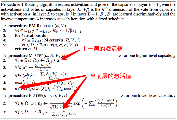
Surprised?
There’s one more thing... readers might notice that according to our definition, we should have \sum_i r_{ij} = 1. Why not simplify it directly? Actually, I don’t know why, but the \text{cost}_j in the paper doesn’t use r_{ij}, but rather a_i^{\text{last}} R_{ij}! That is:
New Dynamic Routing 4: \left\{\begin{aligned} &p_{ij} \leftarrow N(\mathbf{P}_i;\boldsymbol{\mu}_j,\boldsymbol{\sigma}^2_j)\\ &R_{ij} \leftarrow \frac{a_j p_{ij} }{\sum_{j=1}^k a_j p_{ij} }, \quad r_{ij} \leftarrow \frac{a_i^{\text{last}} R_{ij}}{\sum_{i=1}^n a_i^{\text{last}} R_{ij}}\\ &\mathbf{M}_j \leftarrow \sum_{i=1}^n r_{ij}\mathbf{P}_i\\ &\boldsymbol{\sigma}^2_j \leftarrow \sum_{i=1}^n r_{ij}(\mathbf{P}_i-\mathbf{M}_j)^2\\ &\text{cost}_j \leftarrow \left(\beta_u + \sum_{l=1}^d \ln \sigma_j^l \right)\sum_i a_i^{\text{last}} R_{ij} \\ &a_j \leftarrow \text{sigmoid}\left( \lambda \left(\beta_a - \text{cost}_j\right)\right) \end{aligned}\right.
Well, I’m speechless. Hinton can play however he wants. Even if this can be explained away (perhaps meaning this layer’s activation should also be regulated by the previous layer’s activation), it doesn’t offer much enlightenment.
Weight Matrix
Finally, just like in the previous article, we assign a weight matrix \mathbf{W}_{ij} (called the view-invariant matrix) to each pair of indices (i, j), obtaining a "vote matrix" \mathbf{V}_{ij} = \mathbf{P}_i \mathbf{W}_{ij}. Then we perform dynamic routing to get the final algorithm:
New Dynamic Routing (Complete): \left\{\begin{aligned} &p_{ij} \leftarrow N(\mathbf{V}_{ij};\boldsymbol{\mu}_j,\boldsymbol{\sigma}^2_j)\\ &R_{ij} \leftarrow \frac{a_j p_{ij} }{\sum_{j=1}^k a_j p_{ij} }, \quad r_{ij} \leftarrow \frac{a_i^{\text{last}} R_{ij}}{\sum_{i=1}^n a_i^{\text{last}} R_{ij}}\\ &\mathbf{M}_j \leftarrow \sum_{i=1}^n r_{ij}\mathbf{V}_{ij}\\ &\boldsymbol{\sigma}^2_j \leftarrow \sum_{i=1}^n r_{ij}(\mathbf{V}_{ij}-\mathbf{M}_j)^2\\ &\text{cost}_j \leftarrow \left(\beta_u + \sum_{l=1}^d \ln \sigma_j^l \right)\sum_i a_i^{\text{last}} R_{ij} \\ &a_j \leftarrow \text{sigmoid}\left( \lambda \left(\beta_a - \text{cost}_j\right)\right) \end{aligned}\right.
Conclusion
Evaluation
After this analysis, one should feel that this new version of Capsule and its routing algorithm are not complex. The key point of the new paper is the use of GMM to complete the clustering process. GMM is a clustering algorithm based on a probabilistic model. By grasping the "probabilistic model" characteristic and looking for probability-related quantities, it is not difficult to understand the origin of the a_j expression. This is likely the most difficult point in understanding the entire paper. Replacing vectors with matrices is likely just a scheme to reduce computational load and parameter count, without fundamental changes.
However, the new paper inherits the obscure and difficult-to-understand expression style of the old one, combined with chaotic notation, which greatly increases the difficulty of understanding. I once again criticize the authors’ writing.
Of course, there are still some difficult things in the paper where the logic is unclear, such as the replacement of r_{ij} with a_i^{\text{last}} R_{ij} in \text{cost}_j. If anyone has more enlightening ideas, feel free to leave a comment for discussion.
Reflections
By now, I have finally sorted out Matrix Capsules with EM Routing. As for the code, I won’t write it, because I personally don’t particularly like this new Capsule and dynamic routing, and I don’t want to reinvent the wheel.
This is my third article on understanding Capsules. Compared to other articles in Scientific Space, these three are "massive" in length. They carry my thoughts and understanding of Capsules. Each article took several days to write, attempting to combine theory with accessible language as much as possible and to clarify the context. I hope these words help readers understand Capsules more quickly. Of course, my level is limited; if there are any misleading points, criticism is welcome.
Naturally, I hope the authors of Capsule will use more intuitive and enlightening language to introduce their new theory, which would save us science popularizers a lot of work. After all, if Capsule is truly the future of deep learning, how can it be so vague?
Original link: https://kexue.fm/archives/5155