In this article, we analyze Capsule once again.
Overall, the details of the Capsule algorithm are not overly complex; implementing it with a framework by following its process is generally straightforward. Therefore, the difficult part is understanding what Capsule actually does and why it does it, especially the steps involved in Dynamic Routing.
Why do I repeatedly analyze Capsule? This is not merely "reheating old rice," but rather an effort to gain a deeper understanding of the principles behind Capsule. As is well known, Capsule often feels like it contains "too many manual conventions," lacking that intuitive sense of "even if I don’t fully understand it, I believe it should be this way." I hope to clarify the origins and development of Capsule as much as possible, so that we can perceive it as a natural and fluid model, and even apply its logic to other areas.
In "Lifting the Fog: A Delicious Capsule Feast", I first analyzed the results of dynamic routing and then pointed out that the output is a kind of clustering of the input. This "from result to cause" process involved a certain amount of guesswork based on literal interpretation. This time, we do the opposite: we directly confirm that the output is a clustering of the input, and then reverse-engineer what the dynamic routing should be. This significantly reduces the ambiguous components, and the two articles complement each other.
The Capsule Framework
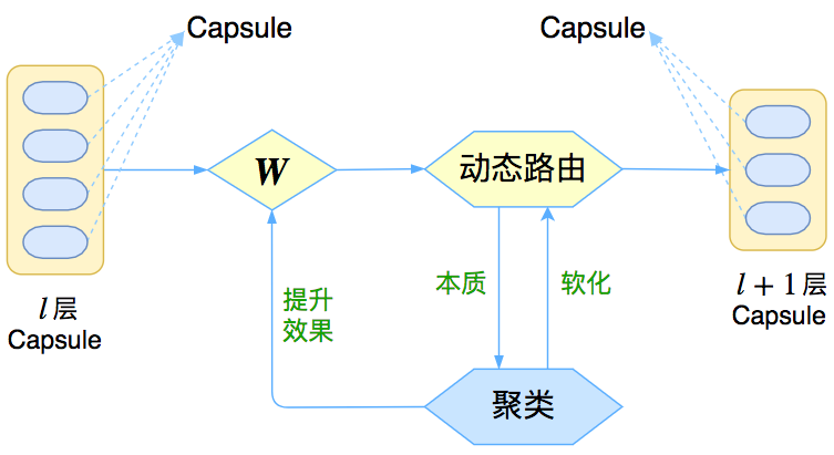
Rather than calling Capsule a specific model, it is better to describe it as a modeling framework. The content of each step within the framework can be flexibly replaced, and the paper published by Hinton is just one use case.
What kind of framework is this?
Feature Representation
In the Capsule model, each feature is represented by a vector (i.e., a Capsule).
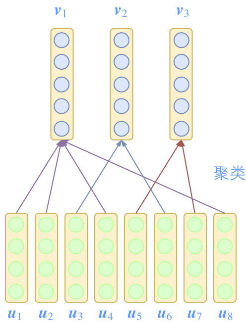
Of course, for readers who follow the news, this is no longer new information. However, one might wonder: what is so special about using vectors to represent features? Isn’t the feature input of a standard neural network already a vector? In a traditional neural network (MLP), each layer’s input is a vector \boldsymbol{x} \in \mathbb{R}^n, and the output is \boldsymbol{y} = \text{Activation}(\boldsymbol{W}\boldsymbol{x} + \boldsymbol{b}) \in \mathbb{R}^k. We treat each component of \boldsymbol{x} as a feature, making each feature a scalar. After "vectorizing" features, the input of each layer becomes \boldsymbol{x} \in \mathbb{R}^{n \times d_x}, and the output is \boldsymbol{y} = \text{Routing}(\boldsymbol{x}) \in \mathbb{R}^{k \times d_y}. Here, the input \boldsymbol{x} is still seen as n features, but each feature is a d_x-dimensional vector; the output \boldsymbol{y} consists of k features, each being a d_y-dimensional vector. From another perspective, the input and output of each MLP layer have changed from a single vector to a set of vectors (a matrix).
Alternatively, we can call this "distributed representation of features." Readers familiar with "distributed representation" might think of word vectors in NLP. Indeed, word vectors were originally called "Distributed Representations." My first reaction to this characteristic of Capsule was its similarity to word vectors. We can use word vectors instead of one-hot encoding to represent a word, which provides much richer information. Furthermore, since all words reside in the same vector space, subsequent processing is more convenient.
In fact, there are similar examples in image processing. As is well known, color images typically have three channels (RGB), each with 256 choices, allowing for 256^3 = 16,777,216 colors. Why not use 17 million unique numbers to represent these colors directly, instead of three groups of 256 numbers? This is also a form of distributed representation, which better captures the diversity of colors (e.g., what is the closest color to red? Some might say orange, others purple, or perhaps pink; a single number struggles to express multiple similarities, whereas grouping allows for it). Furthermore, when we perform continuous convolution operations on an image, the resulting channel dimensions are essentially a distributed representation of image features.
Feature Combination
The second characteristic of Capsule is combining features through clustering.
Combination and Expression
Combining low-level features into high-level features aligns with our cognitive patterns. In NLP, we have the hierarchical combination of "character \to word \to sentence \to paragraph"; in images, we have "point \to line \to surface \to volume." When faced with something new (a high-level feature), we always decompose it into things we are familiar with (low-level features) and then map these things to the new concept in our minds (feature combination).
For us, this process of decomposition and combination does not necessarily have a specific goal; it is simply to understand the new thing in our own way (forming a good feature representation in the brain). This helps explain one of the reasons why Hinton criticizes current deep learning and developed Capsule. He feels that current deep learning models are too task-specific (e.g., an MNIST classification model can only recognize single digits; recognizing multiple digits requires rebuilding the dataset and redesigning/retraining the model). In reality, our fundamental goal is not just to perform tasks, but to form good, universal feature representations through tasks, which is the only way to achieve true artificial intelligence.
Clustering Between Features
So, how is this combination process completed? Imagine why two characters can become a word: it is because these two characters often "cluster" together, and this "cluster" consists only of them. This tells us that features aggregate because they have a clustering tendency, so Capsule integrates clustering algorithms into the model.
Note that the clustering we usually talk about refers to clustering between samples, such as automatically clustering MNIST images into 10 categories or clustering word vectors from Word2Vec into several groups. The object of clustering is a sample (input). Capsule, however, envisions representing the input itself as several feature vectors and then clustering these vectors (clustering between features) to obtain several center vectors. These center vectors are then clustered again, progressing layer by layer to complete the process of abstraction. This is clustering between features.
Now the question arises: since it is clustering, what method is used? And how is that magical Dynamic Routing derived from this clustering method? We will trace this back to K-Means later, but first, let’s finish the main idea.
Feature Significance
Feature combination yields high-level features, but how do we compare the strength of features? Capsule’s answer is: the norm (length). Just as one might look for the "prominent" vector among many, one only needs to see which one is "taller." Therefore, using the norm of a feature vector to measure its "prominence" is a natural choice. Additionally, a bounded measure is desirable, so we squash the feature vector: \text{squash}(\boldsymbol{v}) = \frac{\|\boldsymbol{v}\|^2}{1 + \|\boldsymbol{v}\|^2} \frac{\boldsymbol{v}}{\|\boldsymbol{v}\|} The squashing scheme is not unique, and we won’t expand on it here. However, during my experiments, I found that replacing 1 with 0.5 can improve performance.

To emphasize this meaning of the norm, the model design must cooperate. As shown in the figure, although the norms of the feature vectors \boldsymbol{u}_1, \boldsymbol{u}_2, \boldsymbol{u}_4, \boldsymbol{u}_8 in the class represented by \boldsymbol{v}_1 are relatively small, because there are many members ("many followers"), the norm of \boldsymbol{v}_1 can still be dominant ("great power"). This indicates that for a class to be prominent, it is related to both the number of vectors in the class and the norm of each individual vector. We will see later how Capsule reflects this.
A New Look at K-Means
Since this article emphasizes that Capsule abstracts features through clustering, it is necessary to discuss clustering algorithms in detail. The clustering algorithm used by Capsule is actually a variant of K-Means. There are many clustering algorithms, and theoretically, any could be used; however, embedding a clustering algorithm into Capsule requires some effort.
Clustering Objective
K-Means clustering is essentially a "center-based clustering method"—clustering is about finding class centers. To define a center, we need a measure of similarity. Euclidean distance is common, but it is not the only choice. Therefore, we will introduce K-Means within a more general framework: K-Means aims to partition existing data \boldsymbol{u}_1, \boldsymbol{u}_2, \dots, \boldsymbol{u}_n into k classes unsupervised. The method is to find k cluster centers \boldsymbol{v}_1, \boldsymbol{v}_2, \dots, \boldsymbol{v}_k such that the intra-class interval is minimized: L = \sum_{i=1}^n \min_{j=1}^k d(\boldsymbol{u}_i, \boldsymbol{v}_j) Here d represents the measure of similarity. This formula simply means that each \boldsymbol{u}_i belongs only to the class closest to it, and then all intra-class distances are summed and minimized: (\boldsymbol{v}_1, \dots, \boldsymbol{v}_k) = \arg\min_{(\boldsymbol{v}_1, \dots, \boldsymbol{v}_k)} L
Note: Obviously, the clustering result depends on the specific form of d. This tells us that the difference between unsupervised and supervised learning lies in how we "communicate" with the model. In supervised learning, we convey our intentions through labeled data; in unsupervised learning, we do so by designing an appropriate measure d.
Solving Process
How do we minimize L to find the centers? If you do not wish to follow the derivation in detail, you can skip this section and go directly to the next.
Because L contains the \min operation, calculating its gradient directly is difficult (not impossible, but hard to handle near critical points). In fact, many similar problems remain poorly solved because their loss functions contain \min.
However, we can "soften" this L to make it differentiable. We have a beautiful formula (refer to "Seeking a Smooth Maximum Function"): \begin{aligned} \max(\lambda_1, \lambda_2, \dots, \lambda_n) &= \lim_{K \to +\infty} \frac{1}{K} \ln \left( \sum_{i=1}^n e^{\lambda_i K} \right) \\ &\approx \frac{1}{K} \ln \left( \sum_{i=1}^n e^{\lambda_i K} \right) \end{aligned}
Note: If we take K=1, the term in the parentheses is the denominator of the softmax function. This is the origin of softmax—it is "soft" plus "max."
And we have: \min(\lambda_1, \lambda_2, \dots, \lambda_n) = -\max(-\lambda_1, -\lambda_2, \dots, -\lambda_n) Thus, we get: L \approx -\frac{1}{K} \sum_{i=1}^n \ln \left( \sum_{j=1}^k e^{-K \cdot d(\boldsymbol{u}_i, \boldsymbol{v}_j)} \right) = -\frac{1}{K} \sum_{i=1}^n \ln Z_i Now this approximate loss is smooth and differentiable everywhere. We can attempt to find its gradient: \frac{\partial L}{\partial \boldsymbol{v}_j} \approx \sum_{i=1}^n \frac{e^{-K \cdot d(\boldsymbol{u}_i, \boldsymbol{v}_j)}}{Z_i} \frac{\partial d(\boldsymbol{u}_i, \boldsymbol{v}_j)}{\partial \boldsymbol{v}_j} = \sum_{i=1}^n c_{ij} \frac{\partial d(\boldsymbol{u}_i, \boldsymbol{v}_j)}{\partial \boldsymbol{v}_j} Where: c_{ij} = \text{softmax}_j \Big( -K \cdot d(\boldsymbol{u}_i, \boldsymbol{v}_j) \Big) We have specified that normalization is over the j dimension. To find a minimum, we want \partial L / \partial \boldsymbol{v}_j = 0, but the resulting equation is not easily solvable. Therefore, we can introduce an iterative process. Assuming \boldsymbol{v}_j^{(r)} is the result of the r-th iteration of \boldsymbol{v}_j, we can set: 0 = \sum_{i=1}^n c_{ij}^{(r)} \frac{\partial d(\boldsymbol{u}_i, \boldsymbol{v}_j^{(r+1)})}{\partial \boldsymbol{v}_j^{(r+1)}} If \boldsymbol{v}_j^{(r+1)} can be solved from the above equation, we obtain an iterative format.
Euclidean Distance
Now we can substitute our chosen measure into equation (8). Let’s look at the most basic example: d(\boldsymbol{u}_i, \boldsymbol{v}_j) = \|\boldsymbol{u}_i - \boldsymbol{v}_j\|^2. In this case: \frac{\partial d(\boldsymbol{u}_i, \boldsymbol{v}_j)}{\partial \boldsymbol{v}_j} = 2(\boldsymbol{v}_j - \boldsymbol{u}_i) According to equation (8), we get 0 = 2 \sum_{i=1}^n c_{ij}^{(r)} (\boldsymbol{v}_j^{(r+1)} - \boldsymbol{u}_i), from which we can solve: \boldsymbol{v}_j^{(r+1)} = \frac{\sum_{i=1}^n c_{ij}^{(r)} \boldsymbol{u}_i}{\sum_{i=1}^n c_{ij}^{(r)}} If we take K \to +\infty, then c_{ij}^{(r)} is either 0 or 1, so the above equation means:
\boldsymbol{v}_j^{(r+1)} is the average of those \boldsymbol{u}_i closest to \boldsymbol{v}_j^{(r)}.
This gives us the standard K-Means clustering algorithm.
Inner Product Similarity
Euclidean distance is not suitable for Capsule because the center vector obtained is the average of vectors within the class. Thus, having more vectors in a class does not result in a longer center vector, which fails to satisfy our "more followers, more power" design.
What distance is more suitable? In the paper "Dynamic Routing Between Capsules," there is a passage:
The initial coupling coefficients are then iteratively refined by measuring the agreement between the current output \boldsymbol{v}_j of each capsule, j, in the layer above and the prediction \boldsymbol{\hat{u}}_{j|i} made by capsule i.
The agreement is simply the scalar product a_{ij} = \boldsymbol{v}_j \cdot \boldsymbol{\hat{u}}_{j|i} ...
Corresponding to this article, this roughly means using the inner product \langle \boldsymbol{u}_i, \boldsymbol{v}_j \rangle as a measure of similarity, i.e., d(\boldsymbol{u}_i, \boldsymbol{v}_j) = -\langle \boldsymbol{u}_i, \boldsymbol{v}_j \rangle. But careful thought reveals a problem: such a d is unbounded below! An unbounded function cannot be used as a loss. I was confused by this until one day I realized that \boldsymbol{v}_j could be normalized first before calculating the inner product: d(\boldsymbol{u}_i, \boldsymbol{v}_j) = -\left\langle \boldsymbol{u}_i, \frac{\boldsymbol{v}_j}{\|\boldsymbol{v}_j\|} \right\rangle Now, for a fixed \boldsymbol{u}_i, no matter how \boldsymbol{v}_j changes, d(\boldsymbol{u}_i, \boldsymbol{v}_j) is bounded below. Thus, this d can be used as a loss. Substituting it into equation (8), the final result is: \frac{\boldsymbol{v}_j^{(r+1)}}{\|\boldsymbol{v}_j^{(r+1)}\|} = \frac{\sum_{i=1}^n c_{ij}^{(r)} \boldsymbol{u}_i}{\|\sum_{i=1}^n c_{ij}^{(r)} \boldsymbol{u}_i\|} In other words, \boldsymbol{v}_j^{(r+1)} and \sum_{i=1}^n c_{ij}^{(r)} \boldsymbol{u}_i are in the same direction, though this doesn’t prove they are equal. However, it means we can simply take: \boldsymbol{v}_j^{(r+1)} = \sum_{i=1}^n c_{ij}^{(r)} \boldsymbol{u}_i If we take the limit K \to +\infty, it means:
\boldsymbol{v}_j^{(r+1)} is the sum of those \boldsymbol{u}_i closest to \boldsymbol{v}_j^{(r)}.
Since it is now a sum, it reflects the "more followers, more power" characteristic. (Note that "closest" appears both here and in the Euclidean distance case, but the meaning of "closest" differs because the chosen d is different.)
Note: Derivation of equation (12). \begin{aligned} \frac{\partial \langle \boldsymbol{u}_i, \frac{\boldsymbol{v}_j}{\|\boldsymbol{v}_j\|} \rangle}{\partial \boldsymbol{v}_j} &= \frac{\partial (\boldsymbol{u}_i \cdot \frac{\boldsymbol{v}_j}{\|\boldsymbol{v}_j\|})}{\partial \boldsymbol{v}_j} \\ &= \frac{\boldsymbol{u}_i}{\|\boldsymbol{v}_j\|} + (\boldsymbol{u}_i \cdot \boldsymbol{v}_j) \frac{\partial}{\partial \boldsymbol{v}_j} \frac{1}{\|\boldsymbol{v}_j\|} \\ &= \frac{\boldsymbol{u}_i}{\|\boldsymbol{v}_j\|} - (\boldsymbol{u}_i \cdot \boldsymbol{v}_j) \frac{\boldsymbol{v}_j}{\|\boldsymbol{v}_j\|^3} \end{aligned} Then according to equation (8), we get: 0 = \frac{\sum_{i=1}^n c_{ij}^{(r)} \boldsymbol{u}_i}{\|\boldsymbol{v}_j^{(r+1)}\|} - \left( \sum_{i=1}^n c_{ij}^{(r)} \boldsymbol{u}_i \cdot \boldsymbol{v}_j^{(r+1)} \right) \frac{\boldsymbol{v}_j^{(r+1)}}{\|\boldsymbol{v}_j^{(r+1)}\|^3} Rearranging gives: \sum_{i=1}^n c_{ij}^{(r)} \boldsymbol{u}_i = \left( \sum_{i=1}^n c_{ij}^{(r)} \boldsymbol{u}_i \cdot \frac{\boldsymbol{v}_j^{(r+1)}}{\|\boldsymbol{v}_j^{(r+1)}\|} \right) \frac{\boldsymbol{v}_j^{(r+1)}}{\|\boldsymbol{v}_j^{(r+1)}\|} Taking the norm of both sides: \left\| \sum_{i=1}^n c_{ij}^{(r)} \boldsymbol{u}_i \right\| = \left| \sum_{i=1}^n c_{ij}^{(r)} \boldsymbol{u}_i \cdot \frac{\boldsymbol{v}_j^{(r+1)}}{\|\boldsymbol{v}_j^{(r+1)}\|} \right| = \left\| \sum_{i=1}^n c_{ij}^{(r)} \boldsymbol{u}_i \right\| \times |\cos \theta| Where \theta is the angle between the vector \sum c_{ij}^{(r)} \boldsymbol{u}_i and \boldsymbol{v}_j^{(r+1)}. The equation shows |\cos \theta| = 1, so \theta = 0 or \pi. Since \theta = \pi is a maximum rather than a minimum, \theta = 0, meaning they are in the same direction, yielding equation (12).
Dynamic Routing
After long preparation, the Dynamic Routing algorithm is ready to emerge.
As stated in the first part, each layer in Capsule completes feature combination and abstraction through clustering between features. Clustering requires repeated iteration and is an implicit process. We need to find a smooth, explicit expression for each layer: \boldsymbol{v}_j = \boldsymbol{f}_j(\boldsymbol{u}_1, \dots, \boldsymbol{u}_n) to complete the training of the model. Dynamic routing is the process of writing out this (approximate) explicit expression through iteration.
Basic Steps
Assume the input features of a Capsule are \boldsymbol{u}_1, \boldsymbol{u}_2, \dots, \boldsymbol{u}_n, and the feature vectors of the next layer are \boldsymbol{v}_1, \boldsymbol{v}_2, \dots, \boldsymbol{v}_k, which are the cluster centers of the n vectors from the previous layer. The clustering measure is the normalized inner product mentioned earlier. We can write the iterative process:
Initialize \boldsymbol{v}_j \leftarrow \boldsymbol{v}_j^{(0)}
Iterate r times:
\boldsymbol{v}_j \leftarrow \boldsymbol{v}_j / \|\boldsymbol{v}_j\|
If j = \arg\max_{j=1, \dots, k} \langle \boldsymbol{u}_i, \boldsymbol{v}_j \rangle, then c_{ij} \leftarrow 1, else c_{ij} \leftarrow 0
\boldsymbol{v}_j \leftarrow \sum_i c_{ij} \boldsymbol{u}_i
Return \text{squash}(\boldsymbol{v}_j).
This version is easy to understand, but because of the \arg\max operation, we cannot use gradient descent, which is currently the only method for finding other model parameters. To solve this, we do not take the limit K \to +\infty, but instead take a constant K > 0 and change the algorithm to:
Initialize \boldsymbol{v}_j \leftarrow \boldsymbol{v}_j^{(0)}
Iterate r times:
\boldsymbol{v}_j \leftarrow \boldsymbol{v}_j / \|\boldsymbol{v}_j\|
c_{ij} \leftarrow \text{softmax}_j \Big( \langle \boldsymbol{u}_i, K\boldsymbol{v}_j \rangle \Big)
\boldsymbol{v}_j \leftarrow \sum_i c_{ij} \boldsymbol{u}_i
Return \text{squash}(\boldsymbol{v}_j).
However, this introduces a new parameter K. At first glance, if K is too large, gradients vanish; if K is too small, it’s not accurate enough. But as we will see, we can simply set K=1, because the solution space for K=1 already includes any K. Finally, we get:
Initialize \boldsymbol{v}_j = \boldsymbol{v}_j^{(0)}
Iterate r times:
\boldsymbol{v}_j \leftarrow \boldsymbol{v}_j / \|\boldsymbol{v}_j\|
c_{ij} \leftarrow \text{softmax}_j \Big( \langle \boldsymbol{u}_i, \boldsymbol{v}_j \rangle \Big)
\boldsymbol{v}_j \leftarrow \sum_i c_{ij} \boldsymbol{u}_i
Return \text{squash}(\boldsymbol{v}_j).
Interestingly, the final derived result differs not only from Hinton’s original paper but also from my previous introduction. The most obvious difference is that during the iteration, \boldsymbol{v}_j / \|\boldsymbol{v}_j\| replaces \text{squash}(\boldsymbol{v}_j), and squashing is only performed at the final output. Experiments show that this helps improve feature representation capability; in the numerical experiments of my previous article (single-digit training, double-digit prediction), it reached over 95% accuracy (previously 91%).
Three Symptoms
Is that all? Far from it. We still need to solve several problems.
1. How to perform category initialization? Since clustering results depend on initialization, and good initialization is often half the success. Now that we are embedding clustering into the model, how should each \boldsymbol{v}_j^{(0)} be chosen? If they are initialized identically, the clustering process cannot differentiate them; if initialized randomly, the results won’t be deterministic (even if the center vectors remain the same, the order of classes might change).
2. How to recognize feature order? We know that clustering results are independent of the order of samples. For sample clustering, this is an advantage; however, for feature clustering, it might be inappropriate because different orders of feature combinations may represent different meanings (just as different word orders change a sentence’s meaning). If they all yield the same result, the order information is lost.
3. How to ensure feature expression capability? Dynamic routing treats the upper-layer Capsule as the clustering result of the lower-layer Capsules. Each class may contain multiple feature vectors, but if we only use the center vector to represent the overall feature of the class, will it reduce the expression capability of the upper-layer Capsule?
One Strategy
Interestingly, all three problems can be solved by the same method: adding transformation matrices.
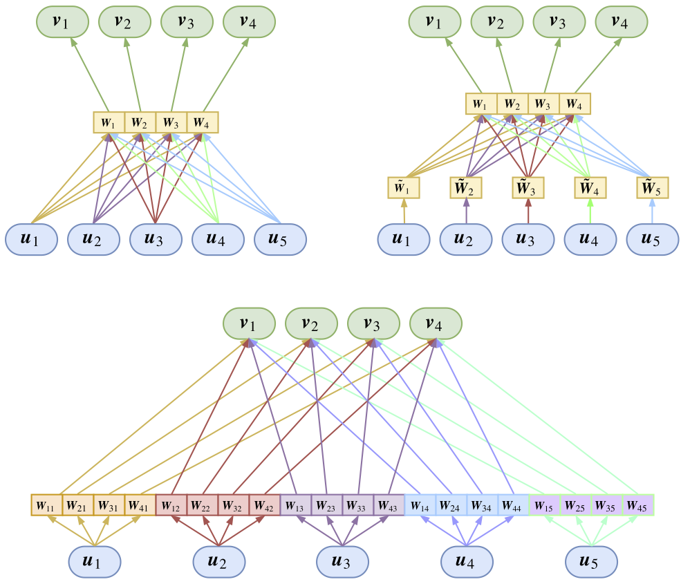
First, for model simplicity, we distribute the sum of all \boldsymbol{u}_i equally to each class as \boldsymbol{v}_j^{(0)}. How do we distinguish between different classes? Before outputting to each class, we assign a transformation matrix \boldsymbol{W}_j to each class to distinguish them. Dynamic routing then becomes:
Initialize \boldsymbol{v}_j \leftarrow \frac{1}{k} \sum_{i=1}^n \boldsymbol{W}_j \boldsymbol{u}_i
Iterate r times:
\boldsymbol{v}_j \leftarrow \boldsymbol{v}_j / \|\boldsymbol{v}_j\|
c_{ij} \leftarrow \text{softmax}_j \Big( \langle \boldsymbol{W}_j \boldsymbol{u}_i, \boldsymbol{v}_j \rangle \Big)
\boldsymbol{v}_j \leftarrow \sum_i c_{ij} \boldsymbol{W}_j \boldsymbol{u}_i
Return \text{squash}(\boldsymbol{v}_j).
This is the shared-weight version of Capsule I mentioned in my previous post. Upon closer inspection, introducing the training matrix \boldsymbol{W}_j is a brilliant move. It not only solves the initialization problem (identical initializations are mapped to different ones by \boldsymbol{W}_j), but also allows \boldsymbol{W}_j to change the dimension of \boldsymbol{u}_i, thereby changing the dimension of the cluster center vector and ensuring its expression capability (it can increase or decrease dimensions). Also, previously we did classification using an inner product with a vector followed by softmax (one vector representing one class); now, it’s equivalent to using a matrix to represent a class, which can express much richer information. Another benefit is that \langle \boldsymbol{W}_j \boldsymbol{u}_i, K\boldsymbol{v}_j \rangle = \langle (K\boldsymbol{W}_j) \boldsymbol{u}_i, \boldsymbol{v}_j \rangle, meaning it already incorporates the parameter K. Thus, we can safely set K=1 without worrying about accuracy—if necessary, the model will adjust \boldsymbol{W}_j to achieve the effect of adjusting K!
Now only one problem remains: recognizing the order of input features. Just like identifying each class, we can assign a transformation matrix \boldsymbol{\tilde{W}}_i to each input to distinguish inputs at different positions. Dynamic routing then becomes:
Initialize \boldsymbol{v}_j \leftarrow \frac{1}{k} \sum_{i=1}^n \boldsymbol{W}_j \boldsymbol{\tilde{W}}_i \boldsymbol{u}_i
Iterate r times:
\boldsymbol{v}_j \leftarrow \boldsymbol{v}_j / \|\boldsymbol{v}_j\|
c_{ij} \leftarrow \text{softmax}_j \Big( \langle \boldsymbol{W}_j \boldsymbol{\tilde{W}}_i \boldsymbol{u}_i, \boldsymbol{v}_j \rangle \Big)
\boldsymbol{v}_j \leftarrow \sum_i c_{ij} \boldsymbol{W}_j \boldsymbol{\tilde{W}}_i \boldsymbol{u}_i
Return \text{squash}(\boldsymbol{v}_j).
If this feels too cumbersome, \boldsymbol{W}_j \boldsymbol{\tilde{W}}_i can be replaced by a single matrix \boldsymbol{W}_{ji}, meaning a transformation matrix is assigned to every pair of indices (i, j). The advantage is a simpler overall structure, but the disadvantage is that the number of matrices increases from n+k to nk:
Initialize \boldsymbol{v}_j \leftarrow \frac{1}{k} \sum_{i=1}^n \boldsymbol{W}_{ji} \boldsymbol{u}_i
Iterate r times:
\boldsymbol{v}_j \leftarrow \boldsymbol{v}_j / \|\boldsymbol{v}_j\|
c_{ij} \leftarrow \text{softmax}_j \Big( \langle \boldsymbol{W}_{ji} \boldsymbol{u}_i, \boldsymbol{v}_j \rangle \Big)
\boldsymbol{v}_j \leftarrow \sum_i c_{ij} \boldsymbol{W}_{ji} \boldsymbol{u}_i
Return \text{squash}(\boldsymbol{v}_j).
This is the fully connected version of dynamic routing. However, we don’t always need to distinguish inputs at different positions. For variable-length inputs, it’s difficult to assign a matrix to every position, which is where the shared version of dynamic routing comes in handy. In general, both the fully connected and shared versions have their uses.
Conclusion
Through these two "lengthy" (and perhaps wordy) blog posts, I have attempted to interpret the Capsule model developed by Hinton. However, my level is limited, and I ask for the reader’s understanding regarding any inaccuracies.
In my personal opinion, Capsule is indeed a novel and promising area of research. It may not necessarily be (though it could be) the future direction of development, but studying it closely is still highly rewarding.
Looking back at the goal stated at the beginning—to make Capsule seem more natural—how do you feel now? My personal feeling is that after this analysis, Capsule is not so detached from everything else, but rather a bold attempt—Hinton boldly integrated the iterative process of clustering into neural networks, thus giving birth to Capsule.
Does this mean we could consider integrating other intuitive algorithms into neural networks to create other interesting things? Let’s wait and see.
Original URL: https://kexue.fm/archives/5112