Unveiling the Mist: A Delicious Feast of Capsules

Feast Features

The characteristic of this Capsule feast is "vector in, vector out," replacing the traditional "scalar in, scalar out." This means the inputs and outputs of neurons have become vectors, which is considered a revolution in neural network theory. But is it really? Haven’t we done "vector in, vector out" tasks before? Yes, and many of them! In NLP, a sequence of word vectors as input can be seen as "vector in." After encoding by RNN/CNN/Attention, it outputs a new sequence, which is "vector out." In current deep learning, there is no shortage of "vector in, vector out" cases, so this alone isn’t the revolution of Capsules.

The revolution of Capsules lies in: It proposes a new "vector in, vector out" transmission scheme, and this scheme is largely interpretable.

If asked why deep learning (neural networks) is effective, I usually answer: Neural networks complete layer-by-layer abstraction of input through stacking, a process that simulates human hierarchical classification to achieve the final output, possessing good generalization capabilities. Indeed, neural networks should work this way, but they cannot tell us that they are definitely doing so. This is the lack of interpretability, one reason why many view deep learning as a black box.

Let’s see how Hinton breaks through this with Capsules.

The Big Bowl Feast

If I were to use a dish to describe Capsules, I would think of the "Big Bowl Feast" (Poon Choi):

Poon Choi is a traditional Hakka dish. It involves placing ingredients layer by layer into a large basin, blending them into a unique flavor. The richest materials are layered in the basin, with those that absorb juices most easily placed at the bottom. As you eat layer by layer, the juices blend, creating a rich and fragrant taste.

Capsules are designed for this "layer-by-layer progression" goal. To be honest, the writing style of the Capsule paper is not very commendable, so I will try to avoid using the same symbols as the paper to prevent further confusion. Let’s look at a diagram.

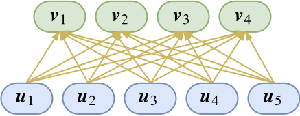
As shown, lower-level capsules and higher-level capsules form connection relationships. Wait, what is a "Capsule"? Actually, as long as you treat a vector as a whole, it is a "Capsule." Yes, you can understand it simply: neurons are scalars, capsules are vectors. It’s that blunt! Hinton’s understanding is: Each capsule represents an attribute, and the vector of the capsule represents the "frame" of this attribute. That is, whereas we previously used a scalar to indicate the presence of a feature (e.g., feathers), we now use a vector to represent not just "if" it exists, but "what kind" (e.g., color, texture). This enriches the expression of individual features.

This reminds me of word vectors in NLP. Previously, we used one-hot encoding to represent a word (just presence). Now we use word vectors, which are richer, representing both presence and semantic similarity. Are word vectors the "Capsules" of NLP? The analogy might be a bit forced, but the essence is correct.

So, how do these capsules operate to reflect "layer-by-layer abstraction" and "layer-by-layer classification"? Let’s look at a part of the connections:

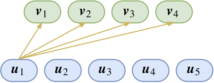
The figure only shows the connections for \boldsymbol{u}_1. This means we already have the feature \boldsymbol{u}_1 (say, feathers), and I want to know which upper-level feature \boldsymbol{v}_1, \boldsymbol{v}_2, \boldsymbol{v}_3, \boldsymbol{v}_4 (say, chicken, duck, fish, dog) it belongs to. We are familiar with classification: isn’t it just an inner product followed by softmax? Thus, based on \boldsymbol{u}_1 alone, we derive the probabilities of it belonging to chicken, duck, fish, or dog as: \big(p_{1|1},p_{2|1},p_{3|1},p_{4|1}\big) = \frac{1}{Z_1}\Big(e^{\langle\boldsymbol{u}_1,\boldsymbol{v}_1\rangle}, e^{\langle\boldsymbol{u}_1,\boldsymbol{v}_2\rangle}, e^{\langle\boldsymbol{u}_1,\boldsymbol{v}_3\rangle}, e^{\langle\boldsymbol{u}_1,\boldsymbol{v}_4\rangle}\Big) \tag{1} We expect p_{1|1} and p_{2|1} to be significantly larger than p_{3|1} and p_{4|1}. However, one feature isn’t enough; we need to synthesize all features. So we repeat this for each \boldsymbol{u}_i, obtaining \big(p_{1|2},p_{2|2},p_{3|2},p_{4|2}\big), \big(p_{1|3},p_{2|3},p_{3|3},p_{4|3}\big), and so on.

The question is, with so many predictions, which one do I choose? And I’m not just doing classification; I want to fuse these features into higher-level ones. Hinton suggests that since the probability distribution for \boldsymbol{u}_i is \big(p_{1|i},p_{2|i},p_{3|i},p_{4|i}\big), I can split this feature into four parts: \big(p_{1|i}\boldsymbol{u}_i, p_{2|i}\boldsymbol{u}_i, p_{3|i}\boldsymbol{u}_i, p_{4|i}\boldsymbol{u}_i\big), and pass them to \boldsymbol{v}_1, \boldsymbol{v}_2, \boldsymbol{v}_3, \boldsymbol{v}_4 respectively. Finally, \boldsymbol{v}_j is the accumulation of features passed from all lower levels: \boldsymbol{v}_j = squash\left(\sum_{i} p_{j|i} \boldsymbol{u}_i\right) = squash\left(\sum_{i} \frac{e^{\langle\boldsymbol{u}_i,\boldsymbol{v}_j\rangle}}{Z_i} \boldsymbol{u}_i\right) \tag{2} Looking from the top down, a Capsule performs classification on each lower feature and integrates the results. Here, \boldsymbol{v}_j should be as close as possible to all \boldsymbol{u}_i (measured by inner product). Thus, looking from the bottom up, \boldsymbol{v}_j is actually a cluster center for the \boldsymbol{u}_i. The core idea of Capsules is that the output is a clustering result of the inputs.

Now, let’s see what this squash thing is.

Fruit Squash

In English, "squash" also refers to a concentrated fruit drink. Let’s taste it. This function appears because Hinton wants Capsules to have a specific property: The length (norm) of the capsule vector represents the probability of the feature.

Actually, I don’t like the term "probability" here because it implies normalization, which is cumbersome. I think it can be called the "salience" of the feature. The larger the norm, the more salient the feature. Since we want a bounded metric for salience, we must compress the norm—"concentration is the essence." Hinton’s compression scheme is: squash(\boldsymbol{x})=\frac{\|\boldsymbol{x}\|^2}{1+\|\boldsymbol{x}\|^2}\frac{\boldsymbol{x}}{\|\boldsymbol{x}\|} \tag{3} The \boldsymbol{x}/\|\boldsymbol{x}\| part is easy to understand (making the norm 1). How to understand the first part? Why this choice? In fact, there are many ways to compress the norm to 0–1, such as: \tanh \|\boldsymbol{x}\|, \quad 1-e^{-\|\boldsymbol{x}\|}, \quad \frac{\|\boldsymbol{x}\|}{1+\|\boldsymbol{x}\|} It’s unclear why Hinton chose this specific one. Perhaps we could explore each? In some experiments, I found that: squash(\boldsymbol{x})=\frac{\|\boldsymbol{x}\|^2}{0.5+\|\boldsymbol{x}\|^2}\frac{\boldsymbol{x}}{\|\boldsymbol{x}\|} works slightly better. This function amplifies norms close to 0, unlike the original function which compresses globally.

However, a question worth considering: Is this compression necessary for intermediate layers? Since dynamic routing is involved, the network already has nonlinearity even without squash. Intuitively, there might be no need to compress features in intermediate layers, just as standard neural networks don’t always use sigmoid to compress to 0–1. This needs to be tested in practice.

Side Dish 1

Let’s return to ordinary neural networks. Activation functions are crucial. A simple tanh-activated fully connected layer in TensorFlow looks like:

y = tf.matmul(W, x) + b
y = tf.tanh(y)

But what if I want to use the inverse function of x = y + \cos y as the activation? That is, you must solve y=f(x) for me.

Mathematicians tell us this inverse is a transcendental function and cannot be expressed with elementary functions. Is this just making things difficult? No, we have iteration: y_{n+1} = x - \cos y_n Choose y_0 = x, substitute it into the formula, and iterate a few times to get an accurate y. If we iterate three times: y = x - \cos(x - \cos(x - \cos x)) In TensorFlow:

y = tf.matmul(W, x) + b
Y = y
for i in range(3):
    Y = y - tf.cos(Y)

If you have "previewed" Capsules, you will find this is very similar to Dynamic Routing.

Side Dish 2

Consider another example common in NLP and some image contexts. Given a sequence of vectors (\boldsymbol{x}_1, \boldsymbol{x}_2, \dots, \boldsymbol{x}_n), I want to integrate them into a single vector \boldsymbol{x} (encoder) for classification.

One might think of LSTM. But I only want to represent it as a linear combination: \boldsymbol{x} = \sum_{i=1}^{n} \lambda_i \boldsymbol{x}_i Here \lambda_i measures the similarity between \boldsymbol{x} and \boldsymbol{x}_i. But before \boldsymbol{x} exists, how can we determine this similarity? Another chicken-and-egg problem. One solution is iteration. We define a softmax-based similarity metric and let: \boldsymbol{x} = \sum_{i=1}^{n} \frac{e^{\langle\boldsymbol{x},\boldsymbol{x}_i\rangle}}{Z} \boldsymbol{x}_i Initially, we know nothing, so we set \boldsymbol{x} to the mean of \boldsymbol{x}_i, substitute it into the right side to calculate a new \boldsymbol{x}, and repeat. This iteration can be embedded in the neural network.

If Side Dish 1 is similar in spirit to Dynamic Routing, Side Dish 2 is similar in both spirit and form. I haven’t seen existing work doing this; it’s just my brainstorming.

The Main Course

With these two side dishes, Dynamic Routing is no longer mysterious. To obtain each \boldsymbol{v}_j, we start by letting them all equal the mean of \boldsymbol{u}_i and then iterate. Simply put, the output is a clustering of the inputs, and since clustering usually requires iterative algorithms, this iteration is called "Dynamic Routing." The details of this routing are not fixed; they depend on the clustering algorithm. For instance, the new paper "MATRIX CAPSULES WITH EM ROUTING" uses a Gaussian Mixture Model.

With this understanding, we can write the Dynamic Routing algorithm used here:

Dynamic Routing Algorithm

Initialize b_{ij}=0
Iterate r times:
\boldsymbol{c}_i \leftarrow softmax(\boldsymbol{b}_i);
\boldsymbol{s}_j \leftarrow \sum_i c_{ij} \boldsymbol{u}_i;
\boldsymbol{v}_j \leftarrow squash(\boldsymbol{s}_j);
b_{ij} \leftarrow \langle\boldsymbol{u}_i, \boldsymbol{v}_j\rangle.
Return \boldsymbol{v}_j.

Here c_{ij} is the p_{j|i} mentioned earlier.

"Wait, I found a mistake! I read the paper, and it should be b_{ij} \leftarrow b_{ij} + \langle\boldsymbol{u}_i, \boldsymbol{v}_j\rangle instead of b_{ij} \leftarrow \langle\boldsymbol{u}_i, \boldsymbol{v}_j\rangle, right?"

Actually, the algorithm above is not wrong—if you accept the derivation in this article and Equation (2), then this iterative process is correct.

"Is Hinton wrong? Do you have the right to challenge Hinton?" Don’t worry, let me analyze what happens with Hinton’s iteration. If we follow Hinton’s algorithm b_{ij} \leftarrow b_{ij} + \langle\boldsymbol{u}_i, \boldsymbol{v}_j\rangle, then after r iterations, it becomes: \boldsymbol{v}_j^{(r)} = squash\left(\sum_i \frac{e^{\langle\boldsymbol{u}_i, \boldsymbol{v}_j^{(0)} + \boldsymbol{v}_j^{(1)} + \dots + \boldsymbol{v}_j^{(r-1)}\rangle}}{Z_i} \boldsymbol{u}_i\right) As \boldsymbol{v}_j^{(r)} approaches the true \boldsymbol{v}_j, we can write: \boldsymbol{v}_j^{(r)} \sim squash\left(\sum_i \frac{e^{r\langle\boldsymbol{u}_i, \boldsymbol{v}_j\rangle}}{Z_i} \boldsymbol{u}_i\right) If we iterate infinitely (r \to \infty), the softmax result becomes either 0 or 1. This means each lower-level capsule connects to exactly one upper-level capsule.

Is this reasonable? I don’t think so. Different categories can share common features; cats and dogs are different but have similar eyes. Some explain this by saying r is a hyperparameter that shouldn’t be too large to avoid overfitting. I don’t know if Hinton thinks so, but if r is just a hyperparameter, it makes Capsules ugly!

Dynamic Routing is already criticized as "unintelligible"; adding a counter-intuitive hyperparameter makes it worse. Conversely, if we use Equation (2) as a starting point, the resulting algorithm fits the clustering idea and is theoretically cleaner, as larger r is always better (limited only by computation), removing the hyperparameter. In fact, I modified the open-source Capsule code with this change and achieved the same results.

I’ll leave the choice to the reader. Personally, I can’t stand theoretical flaws.

Fully Connected Version

Regardless of the version, if \boldsymbol{v}_j is calculated iteratively, are there no parameters? Has backpropagation been abandoned?

Not at all. If that were true, all \boldsymbol{v}_j would be the same. As mentioned, \boldsymbol{v}_j is a cluster center of \boldsymbol{u}_i. To achieve "multi-angle feature viewing," we multiply each capsule by a matrix before passing it to the next layer. Thus, Equation (2) becomes: \boldsymbol{v}_j = squash\left(\sum_{i} \frac{e^{\langle\hat{\boldsymbol{u}}_{j|i},\,\boldsymbol{v}_j\rangle}}{Z_i} \hat{\boldsymbol{u}}_{j|i}\right),\quad \hat{\boldsymbol{u}}_{j|i} = \boldsymbol{W}_{ji}\boldsymbol{u}_i \tag{4} where \boldsymbol{W}_{ji} is the weight matrix to be trained. This is matrix-vector multiplication. The Capsule structure becomes:

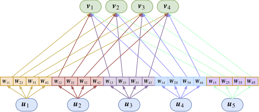
The complete Dynamic Routing algorithm is:

Dynamic Routing Algorithm

Initialize b_{ij}=0
Iterate r times:
\boldsymbol{c}_i \leftarrow softmax(\boldsymbol{b}_i);
\boldsymbol{s}_j \leftarrow \sum_i c_{ij} \hat{\boldsymbol{u}}_{j|i};
\boldsymbol{v}_j \leftarrow squash(\boldsymbol{s}_j);
b_{ij} \leftarrow \langle\hat{\boldsymbol{u}}_{j|i}, \boldsymbol{v}_j\rangle.
Return \boldsymbol{v}_j.

This Capsule layer is equivalent to a fully connected layer in standard networks.

Shared Version

Fully connected layers only handle fixed-length inputs. Since CNNs often handle varying image sizes, the number of extracted features varies, making fully connected Capsules inapplicable. The number of parameter matrices would equal the number of input capsules times output capsules; if the input count is not fixed, we cannot use full connection.

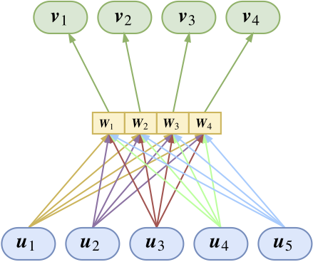
Like weight sharing in CNNs, we need a shared-weight Capsule. For a fixed upper capsule j, the transformation matrix for all lower connections is shared: \boldsymbol{W}_{ji} \equiv \boldsymbol{W}_j.

From the bottom up, all input vectors are mapped by the same matrix, clustered, and output. Repeating this several times outputs several vectors (capsules). From the top down, each matrix is a recognizer for the upper capsule to identify if the lower capsules have that feature. The number of parameters does not depend on the number of input capsules, so it can follow a CNN. For the shared version, Equation (2) becomes: \boldsymbol{v}_j = squash\left(\sum_{i} \frac{e^{\langle\hat{\boldsymbol{u}}_{j|i},\boldsymbol{v}_j\rangle}}{Z_i} \hat{\boldsymbol{u}}_{j|i}\right),\quad \hat{\boldsymbol{u}}_{j|i} = \boldsymbol{W}_{j}\boldsymbol{u}_i \tag{5} The routing algorithm remains the same.

Backpropagation

Although I don’t like the term, we must use it here.

With \boldsymbol{W}_{ji}, how do we train them? Backpropagation. How do dynamic routing and backpropagation work together? It’s simple. Like "Side Dish 1," we embed the iterations (3 steps in the paper) into the model. Formally, it’s like adding three layers. The rest is standard: construct a loss and backpropagate.

Thus, Capsules not only use backpropagation, they only use backpropagation, because dynamic routing is part of the model architecture, not an external optimization algorithm.

What has been achieved?

Capsule provides a new "vector in, vector out" scheme, similar to CNN, RNN, or Attention layers. From Hinton’s perspective, it provides a new scheme based on clustering to replace pooling for feature integration, offering stronger feature expression.

MNIST Classification

Unsurprisingly, Capsules were first tested on MNIST with good results. By perturbing values within a capsule to reconstruct images, it was found that these values represent specific attributes, fulfilling Capsule’s goal.

In classification, Capsules output 10 vectors (one per class), where the norm represents the probability. It treats multi-class classification as multiple binary classifications, using a margin loss: L_c = T_c \max(0, m^+ - \| \boldsymbol{v}_c\|)^2 + \lambda (1 - T_c) \max(0, \| \boldsymbol{v}_c\| - m^-)^2 where T_c = 1 if the class is present. The paper also compares improvements with a reconstruction network.

Overall, the paper’s experiments are a bit rough. Using MNIST is not very challenging (Fashion MNIST would have been better), and the reconstruction network is just two fully connected layers. But for a proof of concept, it suffices.

My Experiment

Since standard CNNs already reach 99%+ accuracy on MNIST, saying Capsules work isn’t very convincing. I designed a new experiment to demonstrate Capsule’s superior ability to integrate features. Capsules don’t just work; they work beautifully.

The experiment:

1. Train a digit recognition model on standard MNIST, but instead of a 10-way softmax, use 10 binary classifications. Both CNN+Pooling and CNN+Capsule can do this.
2. Test the model on a new dataset: randomly pick two images from the test set and concatenate them. See if the model can predict both digits (order doesn’t matter).
The training set is 1-to-1, but the test set is 2-to-2.

The code is on my GitHub. Here is the core part.

First, the CNN part (identical for both models):

input_image = Input(shape=(None,None,1))
cnn = Conv2D(64, (3, 3), activation='relu')(input_image)
cnn = Conv2D(64, (3, 3), activation='relu')(cnn)
cnn = AveragePooling2D((2,2))(cnn)
cnn = Conv2D(128, (3, 3), activation='relu')(cnn)
cnn = Conv2D(128, (3, 3), activation='relu')(cnn)

Then, modeling with standard Pooling + Dense:

cnn = GlobalAveragePooling2D()(cnn)
dense = Dense(128, activation='relu')(cnn)
output = Dense(10, activation='sigmoid')(dense)

model = Model(inputs=input_image, outputs=output)
model.compile(loss=lambda y_true,y_pred: y_true*K.relu(0.9-y_pred)**2 + 0.25*(1-y_true)*K.relu(y_pred-0.1)**2,
              optimizer='adam',
              metrics=['accuracy'])

This model has  270,000 parameters and reaches 99.3%+ on standard MNIST. Now we test the custom task, outputting two accuracies: one for the top two scores, and one where both scores must exceed 0.5.

# Concatenate two test images to form a new test set
idx = range(len(x_test))
np.random.shuffle(idx)
X_test = np.concatenate([x_test, x_test[idx]], 1)
Y_test = np.vstack([y_test.argmax(1), y_test[idx].argmax(1)]).T
X_test = X_test[Y_test[:,0] != Y_test[:,1]] # Ensure different digits
Y_test = Y_test[Y_test[:,0] != Y_test[:,1]]
Y_test.sort(axis=1)

Y_pred = model.predict(X_test)
greater = np.sort(Y_pred, axis=1)[:,-2] > 0.5
Y_pred = Y_pred.argsort()[:,-2:]
Y_pred.sort(axis=1)

acc = 1.*(np.prod(Y_pred == Y_test, axis=1)).sum()/len(X_test)
print u'Accuracy without confidence: %s'%acc
acc = 1.*(np.prod(Y_pred == Y_test, axis=1)*greater).sum()/len(X_test)
print u'Accuracy with confidence: %s'%acc

After testing, accuracy without confidence is  40%, and with confidence is  10%. These are conservative figures.

Now for the Capsule model, replacing the code after the CNN:

capsule = Capsule(10, 16, 3, True)(cnn)
output = Lambda(lambda x: K.sqrt(K.sum(K.square(x), 2)))(capsule)

model = Model(inputs=input_image, outputs=output)
model.compile(loss=lambda y_true,y_pred: y_true*K.relu(0.9-y_pred)**2 + 0.25*(1-y_true)*K.relu(y_pred-0.1)**2,
              optimizer='adam',
              metrics=['accuracy'])

This uses the shared-weight Capsule. The parameter count is also  270,000, and standard MNIST accuracy is  99.3%.

However: On the new test set, the Capsule model achieves over 90% for both accuracies! Even without specific training, Capsules identify the features (digits) with high confidence. Of course, if we trained a standard CNN on double-digit images, it would work well too. The point is that the old architecture lacks generalization. Standard CNN+Pooling needs to be "held by the hand" for every task, while Capsules show an ability to generalize, which is what we truly want.

It looks promising

Capsule aims for an interpretable neural network scheme. From this perspective, it is successful, at least as a "beta" version. Its goal isn’t just accuracy, but an excellent, interpretable representation. My experiment suggests Capsules are closer to the human visual mechanism than pooling.

In fact, using vector norms to represent probability reminds me of wave functions in quantum mechanics, where the norm represents probability. This suggests that the future of Capsules might benefit from concepts in quantum physics.

Urgent need for optimization

Clearly, many areas need optimization. I think the least attractive part isn’t dynamic routing, but the squash function. Is compression necessary for non-output layers? Using norms for probability requires them to be <1, but the sum of two such vectors isn’t necessarily <1, requiring further compression. This feels subjective. We might need tools from manifold analysis or quantum mechanics for a more elegant solution.

Practically, Capsules are slow. Embedding the iterative clustering (dynamic routing) into the network doesn’t add much to the forward pass, but it explodes the backpropagation cost due to complex gradients of composite functions.

Is Backpropagation good?

Hinton wants to abandon backpropagation because it lacks a biological counterpart (requiring precise derivatives).

I disagree. While precise derivatives may not exist in nature, they represent our advancement. Without derivatives, we could still optimize via "trial and interpolation" (e.g., changing \alpha from 3 to 5, seeing the loss drop, then trying 7). This is essentially gradient descent, but it only adjusts one parameter at a time. With millions of parameters, we’d need millions of trials. Calculating the gradient is a superior technique to adjust all parameters at once. Why not use it?

Is Pooling good?

Hinton considers pooling unscientific, but I think its value depends on the context. MNIST (28x28) might not need it, but what about a 1000x1000 image? We see distant things less clearly—isn’t that a form of pooling?

I believe pooling is useful for low-level features. High-level pooling (like Global Pooling) might be problematic as it reduces feature transferability. Even if we avoid pooling, a stride-2 convolution is similar to a stride-1 convolution followed by 2x2 pooling. In my experiment, combining pooling with Capsules did not degrade performance.