A Brief Reading of ``Attention is All You Need'' (Introduction + Code)

Sequence Encoding

The basic approach to NLP using deep learning is to first tokenize the sentence and then convert each word into a corresponding word vector sequence. In this way, each sentence corresponds to a matrix \boldsymbol{X}=(\boldsymbol{x}_1, \boldsymbol{x}_2, \dots, \boldsymbol{x}_t), where \boldsymbol{x}_i represents the word vector (row vector) of the i-th word with dimension d, so \boldsymbol{X} \in \mathbb{R}^{n \times d}. The problem then becomes how to encode these sequences.

The first basic idea is the RNN layer. The RNN approach is simple and recursive: \boldsymbol{y}_t = f(\boldsymbol{y}_{t-1}, \boldsymbol{x}_t) Whether it is the widely used LSTM, GRU, or the recent SRU, they have not deviated from this recursive framework. The RNN structure itself is relatively simple and suitable for sequence modeling, but one obvious disadvantage is that it cannot be parallelized, making it slow—a natural flaw of recursion. Additionally, I personally feel that RNNs cannot learn global structural information well because they are essentially a Markov decision process.

The second idea is the CNN layer. The CNN approach is also quite natural, using a window-based traversal. For example, a convolution with a size of 3 is: \boldsymbol{y}_t = f(\boldsymbol{x}_{t-1}, \boldsymbol{x}_t, \boldsymbol{x}_{t+1}) In Facebook’s paper, pure convolution was used to complete Seq2Seq learning, which is an exquisite and extreme use case of convolution. Readers who are enthusiastic about convolution must read that paper. CNNs are easy to parallelize and can easily capture some global structural information. I personally prefer CNNs; in my current work or competition models, I have tried to replace existing RNN models with CNNs and have formed my own set of experiences, which we will discuss later.

Google’s work provides a third idea: Pure Attention! Attention is all you need! RNNs require step-by-step recursion to obtain global information, so bidirectional RNNs are generally better; CNNs actually only obtain local information and increase the receptive field through stacking. The Attention approach is the most straightforward—it obtains global information in one step! Its solution is: \boldsymbol{y}_t = f(\boldsymbol{x}_{t}, \boldsymbol{A}, \boldsymbol{B}) where \boldsymbol{A}, \boldsymbol{B} are another sequence (matrix). If we take \boldsymbol{A}=\boldsymbol{B}=\boldsymbol{X}, it is called Self-Attention. It means directly comparing \boldsymbol{x}_t with every original word to finally calculate \boldsymbol{y}_t!

Attention Layer

Definition of Attention

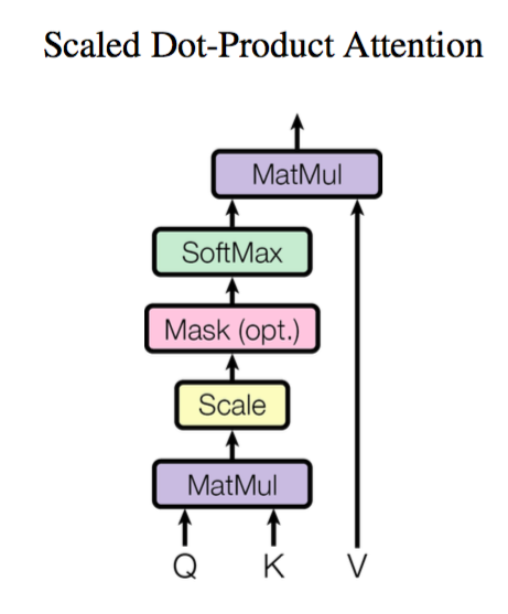
Google’s generalized Attention idea is also a scheme for encoding sequences. Therefore, we can consider it, like RNN and CNN, as a sequence encoding layer.

The generalized framework was given earlier, but Google’s actual solution is very specific. First, it defines Attention as: \text{Attention}(\boldsymbol{Q}, \boldsymbol{K}, \boldsymbol{V}) = \text{softmax}\left(\frac{\boldsymbol{Q}\boldsymbol{K}^{\top}}{\sqrt{d_k}}\right)\boldsymbol{V} Using the same notation as Google’s paper, where \boldsymbol{Q} \in \mathbb{R}^{n \times d_k}, \boldsymbol{K} \in \mathbb{R}^{m \times d_k}, \boldsymbol{V} \in \mathbb{R}^{m \times d_v}. If we ignore the \text{softmax} activation function, it is essentially the multiplication of three matrices of sizes n \times d_k, d_k \times m, m \times d_v, resulting in an n \times d_v matrix. Thus, we can consider this an Attention layer that encodes an n \times d_k sequence \boldsymbol{Q} into a new n \times d_v sequence.

How do we understand this structure? Let’s look at it vector by vector: \text{Attention}(\boldsymbol{q}_t, \boldsymbol{K}, \boldsymbol{V}) = \sum_{s=1}^m \frac{1}{Z} \exp\left(\frac{\langle\boldsymbol{q}_t, \boldsymbol{k}_s\rangle}{\sqrt{d_k}}\right)\boldsymbol{v}_s where Z is the normalization factor. In fact, q, k, v are abbreviations for query, key, value. \boldsymbol{K} and \boldsymbol{V} are in a one-to-one correspondence, like a key-value relationship. The above formula means that through the query \boldsymbol{q}_t, by taking the dot product with each \boldsymbol{k}_s and applying softmax, we obtain the similarity between \boldsymbol{q}_t and each \boldsymbol{v}_s, and then perform a weighted sum to get a d_v-dimensional vector. The factor \sqrt{d_k} plays a regulatory role, ensuring the dot product is not too large (if it’s too large, softmax becomes "hard," i.e., 0 or 1).

In fact, this definition of Attention is not new, but due to Google’s influence, we can consider this definition more formally proposed and treated as a layer; furthermore, this definition is just one form of attention. There are other choices, such as the operation between query and key not necessarily being a dot product (it could be concatenation followed by a dot product with a parameter vector), or the weights not necessarily needing normalization, etc.

Multi-Head Attention

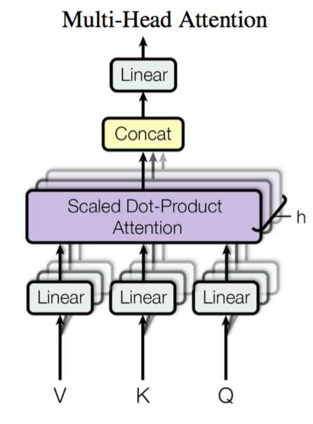
This is a new concept proposed by Google, a refinement of the Attention mechanism. From a formal perspective, it is quite simple: map \boldsymbol{Q}, \boldsymbol{K}, \boldsymbol{V} through parameter matrices, then perform Attention, repeat this process h times, and concatenate the results. It is truly "the Great Way is simple." Specifically: \text{head}_i = \text{Attention}(\boldsymbol{Q}\boldsymbol{W}_i^Q, \boldsymbol{K}\boldsymbol{W}_i^K, \boldsymbol{V}\boldsymbol{W}_i^V) where \boldsymbol{W}_i^Q \in \mathbb{R}^{d_k \times \tilde{d}_k}, \boldsymbol{W}_i^K \in \mathbb{R}^{d_k \times \tilde{d}_k}, \boldsymbol{W}_i^V \in \mathbb{R}^{d_v \times \tilde{d}_v}, and then: \text{MultiHead}(\boldsymbol{Q}, \boldsymbol{K}, \boldsymbol{V}) = \text{Concat}(\text{head}_1, \dots, \text{head}_h) Finally, an n \times (h\tilde{d}_v) sequence is obtained. The so-called “Multi-Head” simply means doing the same thing several times (without sharing parameters) and then concatenating the results.

Position Embedding

However, a little reflection reveals that such a model cannot capture the order of the sequence! In other words, if the rows of \boldsymbol{K} and \boldsymbol{V} are shuffled (equivalent to shuffling the word order in a sentence), the result of Attention remains the same. This indicates that so far, the Attention model is at most a very sophisticated “bag-of-words model.”

This is a serious problem. As we know, for time series, especially for NLP tasks, order is very important information representing local or even global structure. If order information cannot be learned, the effect will be greatly reduced (e.g., in machine translation, it might translate every word but fail to organize them into a coherent sentence).

So Google introduced another trick—Position Embedding. By numbering each position and assigning a vector to each number, and then combining the position vector with the word vector, position information is introduced for each word. This allows Attention to distinguish words at different positions.

Position Embedding is not a new concept; it was also used in Facebook’s “Convolutional Sequence to Sequence Learning.” However, in Google’s work, there are several differences:

1. Previously, Position Embedding appeared in RNN and CNN models, but in those models, it was a supplementary means—“better with it, but not much worse without it”—because RNNs and CNNs themselves can capture position information. But in this pure Attention model, Position Embedding is the sole source of position information, making it a core component rather than just a simple auxiliary.

2. In previous Position Embeddings, the vectors were basically trained based on the task. Google directly provided a formula to construct Position Embedding: \left\{\begin{aligned} &PE_{2i}(p) = \sin\Big(p/10000^{2i/d_{pos}}\Big) \\ &PE_{2i+1}(p) = \cos\Big(p/10000^{2i/d_{pos}}\Big) \end{aligned}\right. This means mapping the position with ID p to a d_{pos}-dimensional position vector, where the i-th element is PE_i(p). Google mentioned in the paper that they compared directly trained position vectors with those calculated by the formula, and the results were similar. Therefore, we prefer using the formula-constructed Position Embedding, which we call Sinusoidal Position Embedding.

3. Position Embedding itself is absolute position information, but in language, relative position is also important. A key reason Google chose the aforementioned formula is: since \sin(\alpha+\beta) = \sin\alpha\cos\beta + \cos\alpha\sin\beta and \cos(\alpha+\beta) = \cos\alpha\cos\beta - \sin\alpha\sin\beta, the vector at position p+k can be expressed as a linear transformation of the vector at position p. This provides the possibility of expressing relative position information.

There are several options for combining position vectors and word vectors: they can be concatenated into a new vector, or the position vector can be defined to be the same size as the word vector and then added together. Both Facebook’s and Google’s papers use the latter. Intuitively, addition might lead to information loss and seem undesirable, but Google’s results show that addition is a very good scheme. It seems my understanding is not yet deep enough.

Also, although the paper gives the Position Embedding in an interleaved \sin, \cos form, this interleaved form has no special significance. You can rearrange it in any way (e.g., \sin first, then \cos), for the following reasons:

1. If your Position Embedding is concatenated to the original word vector, whether \cos and \sin are connected sequentially or interleaved makes no difference, because the next step is just a transformation matrix.

2. If your Position Embedding is added to the original word vector, the two methods might seem different. However, it should be noted that word vectors themselves have no local structure. That is, for a 50-dimensional word vector, if you shuffle every dimension (applying the same shuffle to all vectors), it is still equivalent to the original word vector. Since the object being added (the word vector) has no local structure, there is no need to emphasize the local structure (interleaved connection) of the object being added (Position Embedding).

Some Shortcomings

At this point, the Attention mechanism has been basically introduced. The advantage of the Attention layer is its ability to capture global connections in one step because it directly compares sequences pairwise (at the cost of \mathcal{O}(n^2) computation, though this is not too severe as it is pure matrix operation). In contrast, RNNs need step-by-step recursion, and CNNs need stacking to expand the receptive field. This is a clear advantage of the Attention layer.

The rest of Google’s paper describes how it is applied to machine translation, which is a matter of application and hyperparameter tuning that we won’t focus on here. Of course, Google’s results show that using a pure attention mechanism in machine translation achieves the best results currently, which is indeed brilliant.

However, I still want to talk about some shortcomings of the paper itself and the Attention layer.

1. The paper is titled “Attention is All You Need,” so it deliberately avoids the terms RNN and CNN. But I think this approach is too deliberate. In fact, the paper specifically names a “Position-wise Feed-Forward Network,” which is actually a 1D convolution with a window size of 1. It feels like they created a new name just to avoid mentioning convolution, which is a bit disingenuous (or perhaps I am over-speculating).

2. Although Attention has no direct connection with CNN, it actually draws heavily on CNN ideas. For example, Multi-Head Attention is just doing Attention multiple times and concatenating, which is consistent with the idea of multiple kernels in CNN. Also, the paper uses residual structures, which also originate from CNN networks.

3. It cannot model position information well, which is a fundamental flaw. Although Position Embedding can be introduced, I believe this is only a mitigation and does not fundamentally solve the problem. For example, using this pure Attention mechanism to train a text classification or machine translation model should work well, but for sequence labeling (segmentation, entity recognition, etc.), the effect is not as good. Why does it work well for machine translation? I think it’s because machine translation doesn’t emphasize word order extremely strictly, so the position information from Position Embedding is sufficient. Additionally, the evaluation metric BLEU does not particularly emphasize word order.

4. Not all problems require long-range, global dependencies; many problems only depend on local structures, where pure Attention might not be ideal. In fact, Google seems to have realized this, as the paper mentions a restricted version of Self-Attention (though it might not be used in the main text), which assumes the current word only relates to the r words before and after it. Thus, attention only occurs within these 2r+1 words, making the computation \mathcal{O}(nr) and capturing local structure. But obviously, this is just the concept of a convolution window!

Through the above discussion, we can see that treating Attention as a separate layer and mixing it with CNN and RNN structures should better integrate their respective advantages, rather than claiming “Attention is All You Need” as Google’s paper does, which is a bit of an overcorrection (too much "bravado") and actually impossible to achieve. Regarding the paper’s work, perhaps lowering the stance and calling it “Attention is All Seq2Seq Need” (which is still a bold claim) would have garnered more affirmation.

Code Implementation

Finally, to make this article practically useful, I have tried to provide the implementation code for the Multi-Head Attention described in the paper. Readers in need can use it directly or refer to it for modifications.

Note that although the meaning of Multi-Head is simple—repeat several times and concatenate—you cannot write the program according to this logic, as it would be very slow. Tensorflow does not automatically parallelize operations like:

a = tf.zeros((10, 10))
b = a + 1
c = a + 2

where the calculations of b and c are serial even though they don’t depend on each other. Therefore, we must combine Multi-Head operations into a single tensor operation, as multiplication within a single tensor is automatically parallelized.

Additionally, we need to mask the sequence to ignore the influence of padding. General masking sets the padded parts to zero, but masking in Attention should subtract a large integer before the softmax (so that after softmax, it is very close to 0). These details are implemented in the code.

from __future__ import print_function
from keras.preprocessing import sequence
from keras.datasets import imdb
from attention_keras import *

max_features = 20000
maxlen = 80
batch_size = 32

print('Loading data...')
(x_train, y_train), (x_test, y_test) = imdb.load_data(num_words=max_features)
print(len(x_train), 'train sequences')
print(len(x_test), 'test sequences')

print('Pad sequences (samples x time)')
x_train = sequence.pad_sequences(x_train, maxlen=maxlen)
x_test = sequence.pad_sequences(x_test, maxlen=maxlen)
print('x_train shape:', x_train.shape)
print('x_test shape:', x_test.shape)

from keras.models import Model
from keras.layers import *

S_inputs = Input(shape=(None,), dtype='int32')
embeddings = Embedding(max_features, 128)(S_inputs)
# embeddings = SinCosPositionEmbedding(128)(embeddings) # Adding Position_Embedding can slightly improve accuracy
O_seq = Attention(8,16)([embeddings,embeddings,embeddings])
O_seq = GlobalAveragePooling1D()(O_seq)
O_seq = Dropout(0.5)(O_seq)
outputs = Dense(1, activation='sigmoid')(O_seq)

model = Model(inputs=S_inputs, outputs=outputs)
model.compile(loss='binary_crossentropy',
              optimizer='adam',
              metrics=['accuracy'])

print('Train...')
model.fit(x_train, y_train,
          batch_size=batch_size,
          epochs=5,
          validation_data=(x_test, y_test))

Conclusion

Thanks to Google for providing such a wonderful use case, which has broadened my horizons and deepened my understanding of Attention. Google’s achievement reflects the philosophy of “the Great Way is simple” to some extent and is indeed a rare masterpiece in NLP. This article has discussed Google’s work in a humble manner, hoping to help readers better understand Attention. Finally, I welcome any suggestions and criticisms.

When reposting, please include the original address of this article: https://kexue.fm/archives/4765

For more details on reposting, please refer to: Scientific Space FAQ