Friends who have studied real analysis always know that there is something called the Lebesgue integral, which is claimed to be an improved version of the Riemann integral. Although there is a saying among students that “study real analysis ten times, and functional analysis will make your heart turn cold,” we are usually in a fog when learning real analysis. However, by the end, under the “irrigation” of the teachers, we become familiar with some conclusions, such as “a Riemann integrable function (on a finite interval) is also Lebesgue integrable.” Simply put, “the Lebesgue integral is stronger than the Riemann integral.” So, the question arises: exactly where is it stronger? And why is it stronger?
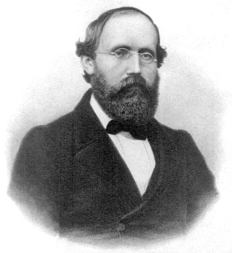
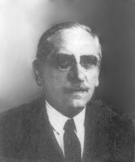
I did not fully understand this question when I was studying real analysis, and I kept it aside until recently when I carefully read Revisiting Calculus. I finally gained some insight. By the way, Professor Qi Minyou’s Revisiting Calculus is truly excellent and worth reading.
Born from the same root, why are we so eager to destroy each other?
As readers who have studied real analysis know, one of the most obvious differences between the Lebesgue integral and the Riemann integral, as two different theories describing integration, is: the Riemann integral partitions the domain, while the Lebesgue integral partitions the codomain (range). At first glance, it seems like Lebesgue was trying to oppose Riemann—you say partition the domain, I refuse; I prefer to partition the range.
So, what is the truth? Is it really just a matter of being “eager to destroy each other”? Not at all. Partitioning the range indeed helps improve the deficiencies of the Riemann integral. Why is partitioning the range stronger than partitioning the domain? The popular explanation is this: The Riemann integral partitions the domain. However, for functions that oscillate wildly, even if the partition is very fine, the oscillation within a tiny interval remains intense (a typical example is the Dirichlet function). In such cases, the Riemann integral cannot be defined. That is to say, the Riemann integral is suitable for locally smooth functions. The Lebesgue integral, by partitioning the range, ensures that within a small interval of the range, there won’t be large oscillations because the range itself is restricted, giving the function no chance to oscillate wildly. Therefore, it can integrate functions that oscillate very intensely.
Others laugh at my madness, I laugh at their lack of insight
Lebesgue speaks: “What you said is somewhat on track, but you haven’t reached my original intention. First, let me declare, I am not trying to oppose the great Master Riemann...” (Purely my own fictional dialogue ^_^)
In fact, the shortcomings of the Riemann integral can be traced back to the “method of exhaustion” of ancient Greece two thousand years ago. For example, to find the area of a circle, they used circumscribed regular n-gons and inscribed regular n-gons to obtain the upper and lower bounds of the circle’s area. Then, by taking the limit, they found that the upper and lower bounds were equal, thus determining the area. That is to say, to find the area of an irregular shape, you divide it into pieces, approximate each piece with a familiar shape (rectangle, triangle), calculate the approximate area, and finally take the limit of the partition. The entire process is: Finite partitioning — approximate summation — taking the limit.
The problem lies in “finite partitioning”! To obtain the upper bound of the area, we need to cover it with a finite number of simple shapes, and to obtain the lower bound, we need a finite number of simple shapes covered by the figure. In short, it is always “finite.” This finiteness is reliable for continuous intervals but is not feasible for general point sets. For example, consider the set of rational numbers in [0, 1]. Readers can imagine the set of all rational points in the interval [0, 1] on the number line and consider its length. Readers who have studied set theory know that the cardinality of real numbers in [0, 1] is uncountable, while rational numbers are countable—meaning there are far more real numbers than rational numbers. Therefore, if we consider the length of the set of all real points in [0, 1] to be 1, then naturally, the length of the set of all rational points in [0, 1] should be 0. However, the finite partitioning used in Riemann integration cannot reach this conclusion.
If we use a finite number of intervals to cover all rational numbers in [0, 1] (covering to get the upper bound), because rational numbers are dense, one can imagine that the total length of these finite intervals will not be less than 1. That is, the upper bound of the total length of all rational numbers in [0, 1] will not be less than 1. However, because any interval contains irrational numbers, rational numbers cannot cover any interval (no matter how small the length). From this perspective, the lower bound of the total length of rational numbers will not be greater than 0. This shows that the result does not converge! This is the problem brought by finite partitioning.
Thus, Lebesgue was very clever; he abandoned finite partitioning from the beginning and used countable partitioning to define measure. Of course, I don’t intend to use the strict language of textbooks here, just the general idea: Taking one dimension as an example, if a subset of real numbers can be covered by countably many intervals, then the total length of these intervals is its upper bound of measure. If it can cover countably many intervals, then the total length of these intervals is its lower bound of measure. If the limits of the upper and lower bounds are equal, then it is a measurable set.
Great wisdom appears foolish, great skill appears clumsy
In fact, with countable partitioning, we can attempt to improve the Riemann integral. Because we have countable partitioning, we can divide a function into several parts to handle—for example, normal points and abnormal points—and the abnormal parts can be further subdivided into the first type of abnormality, the second type, and so on, processing them one by one. Countable partitioning is their foundation. For instance, if we want to pick out all rational points and keep the total length of the intervals arbitrarily small, we must use countably many intervals; a finite number of intervals cannot do it.
The question arises again: how do we distinguish whether a point is normal or abnormal? For the Riemann integral, abnormal points are those where the oscillation is intense. In other words, we must consider the range! This is where another clever point of Lebesgue is reflected: Instead of distinguishing the abnormal points in the Riemann integral one by one, just partition the range directly.
At first glance, partitioning the range seems like a very non-intuitive and clumsy method because it makes the intervals of the domain complex. In fact, this is a move of “great wisdom appearing foolish,” because countable partitioning has already been defined, and any complex domain can be handled. Thus, combining “countable partitioning” and “range partitioning,” the theory called the Lebesgue integral took shape, and the rest is theoretical detail. By the way, Because countable partitioning is used, the Lebesgue integral naturally possesses countable additivity, while correspondingly, the Riemann integral only has finite additivity.
From the discussion in this section, it can be seen that Lebesgue measure and the Lebesgue integral can handle cases with countably many abnormal points (discontinuities). Therefore, it is obvious that if the number of abnormal points is uncountable, both Lebesgue measure and the Lebesgue integral fail. So, to construct an example of a Lebesgue non-measurable set, one must increase the number of abnormal points to uncountable. The “Vitali set,” which is Lebesgue non-measurable, is constructed this way. It starts from the uncountability of real numbers and the countability of rational numbers, uses rational numbers as a reference, and divides the real numbers in [0, 1] into countably many sets, each of which is uncountable. But the problem is, what is the measure of each set? If it is 0, how can the sum of countably many zeros be 1? If it is not 0, then the sum of countably many positive numbers is even less likely to be 1. Therefore, in any case, countable additivity is not satisfied.
Extreme rigidity cannot last, extreme softness cannot defend, things turn into their opposites
From this, it seems that the Lebesgue integral is indeed stronger than the Riemann integral, as it was originally designed to target the “Achilles’ heel” of the Riemann integral.
In life, we often encounter examples where if the purpose is too strong, it often backfires. Since the Lebesgue integral so pointedly “restrains” the Riemann integral, could it instead have some shortcomings that the Riemann integral does not have?
First, an obvious point is that the linear properties of the Lebesgue integral become less obvious. A large portion of Lebesgue integration theory is spent proving that \int_a^b f(x)dx + \int_a^b g(x)dx = \int_a^b [f(x)+g(x)]dx whereas this is almost obviously true in Riemann integration. This might be one of the reasons why the Riemann integral is used to define integration when first learning calculus—because it is intuitive.
Furthermore, there are some insurmountable shortcomings. Inspired by the Dirichlet function, we can easily construct examples that are Riemann non-integrable but Lebesgue integrable. Is there any example of the opposite? The answer is yes!
We can find the problem in the “countable partitioning” of the Lebesgue integral mentioned earlier. The Lebesgue integral allows countably many intervals to approximate from the start and then calculates the sum of the function over these countably many intervals. Because it directly uses countable partitioning and then sums, without a specific sequence, this summation process does not consider order. We know that a series whose sum does not depend on the order of terms is what we call an absolutely convergent series. Thus, we can sense that the Lebesgue integral must be (in the sense of the Riemann integral) absolutely convergent.
However, many practical integrals are not absolutely convergent. For example, the integral \int_{-\infty}^{+\infty} \frac{\sin x}{x}dx is only conditionally convergent and not absolutely convergent. Therefore, for the Lebesgue integral, it is non-integrable! But for the Riemann integral, by understanding it as \lim_{N\to\infty}\int_{-N}^{+N} \frac{\sin x}{x}dx one can obtain a meaningful result. This feels somewhat ironic: “Countable partitioning” was originally introduced to improve the weaknesses of the Riemann integral, but here, it becomes its own weakness. It seems that “things turn into their opposites,” and there is no perfect solution. Please consider the following example.
Return to the original intention, don’t forget the starting point
Let’s talk about probability theory and consider the following question:
If a number is randomly selected from the natural numbers, what is the probability of selecting 1?
Is it obviously 0? Our intuition says 0, but according to the modern axiomatic definition, this probability does not exist!! This probability cannot be defined!!
Let’s look at the axiomatic definition of probability:
For every event A, if the function P(A) satisfies the following conditions, then P(A) is the probability of A:
Non-negativity, i.e., P(A) is non-negative;
Normality, i.e., for the certain event S, P(S)=1;
Countable additivity, i.e., the probability of the union of mutually exclusive events is the sum of their probabilities.
The first two points are not the main issue; the key is the third point: countable additivity! If we believe the probability of selecting 1 is 0, then the probability of selecting 2 is also 0, and the probability of selecting any given natural number is 0. Since the sum of countably many zeros is still 0, the probability of selecting a natural number from the set of all natural numbers would be 0 instead of 1! In other words, countable additivity is not satisfied.
From this perspective, it seems we cannot discuss probability on a countable set. Does this mean mathematicians in the branch of “probabilistic number theory” are just talking nonsense? Is that really the case?
Where did the axiomatic definition of probability, especially countable additivity, come from? If you compare it with the axiomatic definition of Lebesgue measure, you will find that, apart from different terminology, they are almost identical. Countable additivity is also a requirement for measure! In fact, probability defined this way is just a type of Lebesgue measure, or rather, the definition of probability basically copied the definition of measure. The example above shows that countable additivity is truly something that people both love and hate.
However, we still feel it is necessary to discuss probability in the set of natural numbers. What should we do? Probabilistic number theory says: We first discuss within the range of natural numbers not exceeding N, and then let N tend to infinity. Well, doesn’t this return to the Riemann integral’s approach of finite partitioning followed by taking a limit?
It seems that “overthrowing Riemann” is truly impossible...
When reprinting, please include the original address: https://kexue.fm/archives/4083
For more detailed reprint matters, please refer to: Scientific Space FAQ