During the summer vacation, I participated in the Core Entity Recognition competition jointly organized by Baidu and Xi’an Jiaotong University. The final results were quite good, so I am recording the process here. While the model’s performance might not be the absolute best, its strength lies in being end-to-end and highly transferable, which I believe will be of reference value to others.
The theme of the competition is "Core Entity Recognition," which actually involves two tasks: Core Recognition + Entity Recognition. Although these two tasks are related, they are generally handled separately in traditional Natural Language Processing (NLP) pipelines. This competition required combining the two. If we only look at "Core Recognition," it is a traditional keyword extraction task. However, traditional purely statistical approaches (such as TF-IDF extraction) do not work well here because a core entity in a single sentence might appear only once. In such cases, statistical estimates are unreliable, and it is better to understand the sentence from a semantic perspective. I initially started with "Core Recognition" using a method similar to QA systems:
1. Tokenize the sentence and train word vectors using Word2Vec;
2. Use a Convolutional Neural Network (CNNs often perform better than RNNs on this type of extractive problem) to produce an output with the same dimension as the word vectors;
3. The loss function is the cosine similarity between the output vector and the core word vector of the training sample.
To find the core words of a sentence, I only needed to calculate an output vector for each sentence and then compare its cosine similarity with the vector of each word in the sentence, sorting them in descending order. The obvious advantage of this method is its fast execution speed. Ultimately, I achieved an accuracy of 0.35 on the public evaluation set with this model. Later, feeling it was difficult to improve further, I abandoned this approach.
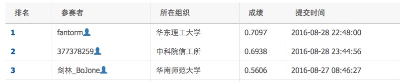
Why did I give up? In fact, while this approach performed well in "Core Recognition," its fatal flaw was its dependency on segmentation results. Tokenization systems often split core entities composed of long words. For example, "Zhu Family Garden" might be split into "Zhu Family / Garden." Once split, it becomes much harder to integrate them. Consequently, I referred to the article "Chinese Word Segmentation Series 4: Seq2seq Character Tagging Based on Bidirectional LSTM" and adopted a word tagging approach, as this method does not rely heavily on segmentation quality. Eventually, I achieved an accuracy of 0.56 using this method.
The main steps were:
1. Tokenize the sentence and train word vectors using Word2Vec;
2. Convert the output into a 5-tag labeling problem:
b(start of core entity),m(middle),e(end),s(single-word core entity), andx(non-core entity part);3. Use a double-layer Bidirectional LSTM for prediction and the Viterbi algorithm for sequence labeling.
Finally, it is worth mentioning that according to this logic, core entity recognition can even be done without tokenization. However, generally speaking, tokenization still yields better results and helps reduce sentence length (a 100-character sentence becomes a 50-word sentence), which reduces the number of model parameters. Here, we only need a simple tokenization system without requiring built-in new word discovery features.
Transfer Learning
However, before using this approach, I was very uncertain about its
final effect. The main reason was: Baidu provided 12,000 training samples but
had 200,000 test samples. With such a disparate ratio,
it seemed difficult for the performance to be good. Additionally, there
are 5 tags, and compared to the x tag, the quantities of
the other four tags are very small. With only 12,000 training samples,
there appeared to be a data insufficiency problem.
Of course, practice is the sole criterion for testing truth. The first test of this approach reached an accuracy of 0.42, far higher than the CNN approach I had carefully tuned for over half a month. So, I continued with this logic. Before proceeding, I analyzed why this approach worked well. I believe there are two main reasons: one is "Transfer Learning," and the other is LSTM’s powerful ability to capture semantics.
Traditional data mining training models are built purely on the training set. However, we can hardly guarantee that the training set and the test set are consistent; specifically, it is hard to assume that the distributions of the training and test sets are the same. Consequently, even if the model training effect is very good, the test performance might be a mess. This is not necessarily caused by overfitting but by the inconsistency between the training and test sets.
One way to solve (or alleviate) this problem is "Transfer Learning." Transfer Learning is now a comprehensive modeling strategy. Generally, it has two schemes:
1. Pre-modeling transfer learning: Put the training set and test set together to learn the features used for modeling. The features obtained this way already contain information from the test set.
2. Post-modeling transfer learning: If the test performance is decent (e.g., 0.5 accuracy), to improve it, you can take the test set along with its predicted results as training samples and re-train the model with the original training samples.
You might be confused about the second point: aren’t the predicted results of the test set incorrect? Can inputting wrong results improve accuracy? Tolstoy said, "All happy families are alike; each unhappy family is unhappy in its own way." Applying this here, I would say, "Correct answers are all the same; incorrect answers are each wrong in their own way." That is to say, if the second point of training is performed, the correct answers in the test set will have a cumulative effect because they result from the same correct patterns. However, incorrect answers have different error patterns. If the model parameters are limited and do not overfit, the model will smooth out these error patterns and lean toward the correct answers. Whether this understanding is accurate is for the reader to judge. Additionally, if new prediction results are obtained, one can take only the identical predictions from two iterations as training samples, which increases the proportion of correct answers.
In this competition, transfer learning was reflected in:
1. Training Word2Vec using both training and test corpora so that word vectors capture the semantics of the test corpus;
2. Training the model with the training corpus;
3. After obtaining the model, predicting on the test corpus and training a new model using the predictions combined with the training corpus;
4. Predicting with the new model, which usually yields an improvement;
5. Comparing the results of two predictions; if they are identical, the prediction is likely correct. Use these "likely correct" test results to train the model;
6. Predicting with the updated model;
7. If desired, repeat steps 4, 5, and 6.
Bidirectional LSTM
The main model structure:
'''
Train the model using the latest version of Keras with GPU acceleration.
The Bidirectional function currently requires the GitHub version.
'''
from keras.layers import Dense, LSTM, Lambda, TimeDistributed, Input, Masking, Bidirectional
from keras.models import Model
from keras.utils import np_utils
from keras.regularizers import activity_l1 # Use L1 regularization to make output sparser

sequence = Input(shape=(maxlen, word_size))
mask = Masking(mask_value=0.)(sequence)
blstm = Bidirectional(LSTM(64, return_sequences=True), merge_mode='sum')(mask)
blstm = Bidirectional(LSTM(32, return_sequences=True), merge_mode='sum')(blstm)
output = TimeDistributed(Dense(5, activation='softmax', activity_regularizer=activity_l1(0.01)))(blstm)
model = Model(input=sequence, output=output)
model.compile(loss='categorical_crossentropy', optimizer='adam', metrics=['accuracy'])
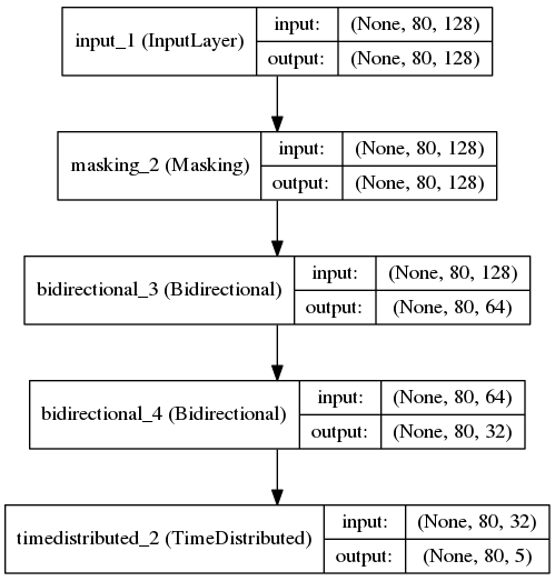
I used a double-layer Bidirectional LSTM (I also tried a single layer, but an extra layer performed better), preserved the output of the LSTM at each step, and applied a softmax to each output. The entire process is essentially like a word segmentation system.
Of course, the quality of this model depends largely on the quality of the word vectors. After multiple adjustments, I found the following Word2Vec parameters to be essentially optimal:
word2vec = gensim.models.Word2Vec(dd['words'].append(d['words']),
                                  min_count=1,
                                  size=word_size,
                                  workers=20,
                                  iter=20,
                                  window=8,
                                  negative=8,
                                  sg=1)
That is, skip-gram performs better than CBOW, negative sampling is better than hierarchical softmax, the number of negative samples should be moderate, and the window size should be moderate. Of course, this "optimal" configuration is based on my "intuitive feeling" after multiple manual adjustments; everyone is welcome to perform more tests.
About the Competition
I actually noticed this competition by Baidu and Xi’an Jiaotong University last year, but I was at a novice level then and couldn’t handle such a difficult task. I tried it this year and felt I gained a lot.
First of all, the competition is held by Baidu, which is attractive in itself because getting recognition from Baidu feels like a significant achievement. I look forward to such competitions and hope Baidu’s competitions get better and better. Secondly, through this process, I gained a deeper understanding of language models, deep network construction, and usage, such as how CNNs are used for language tasks, which language tasks they are suitable for, and the preliminary use of seq2seq.
Coincidentally, this was an NLP task, and the previous Teddy Cup was an image task. Combining the two, I have gone through the basic tasks of both NLP and Computer Vision. I now feel more confident and grounded in handling these types of tasks.
Complete Code
Training set link: https://pan.baidu.com/s/1i457nkL Password: stkp
Documentation
Core Entity Recognition based on Transfer Learning and Bidirectional LSTM
==============================================================
General Steps (corresponding to train_and_predict.py)
==============================================================1. Tokenize both training and test corpora, currently using Jieba;
2. Convert to a 5-tag labeling problem and construct training labels;
3. Train the Word2Vec model using both training and test corpora;
4. Train the labeling model using double-layer Bi-LSTM based on seq2seq ideas;
5. Predict with the model; accuracy fluctuates around 0.46–0.52;
6. Treat prediction results as labeled data and re-train the model with training data;
7. Predict with the new model; accuracy fluctuates around 0.5–0.55;
8. Compare two prediction results, take the intersection as labeled data, and re-train;
9. Predict with the updated model; accuracy stays around 0.53–0.56.==============================================================
Environment:
==============================================================Hardware:
1. 96G RAM (actually uses about 10G)
2. GTX960 GPU (for acceleration)Software:
1. CentOS 7
2. Python 2.7
3. Jieba, Numpy, SciPy, Pandas, Keras (GitHub version), Gensim, H5PY, tqdm==============================================================
File Usage:
==============================================================
train_and_predict.pycontains the entire process. As long as the "unopened validation data" format is the same as "opendata_20w," you can run it to generate models and result files (result1.txt to result5.txt).
train_and_predict.py (Code is not cleaned up, for reference only)
#! -*- coding:utf-8 -*-

'''
Core Entity Recognition based on Transfer Learning and Bi-LSTM
'''

import numpy as np
import pandas as pd
import jieba
from tqdm import tqdm
import re

d = pd.read_json('data.json') # Training data preprocessed into standard JSON
d.index = range(len(d))
word_size = 128
maxlen = 80

'''
Modified tokenization function:
1. English and numbers are not split.
2. Content in double angle brackets is not split.
3. Content in double quotes under 10 chars is not split.
4. Other characters replaced by spaces.
5. Use Jieba without HMM.
'''

not_cuts = re.compile(u'([\da-zA-Z \.]+)|<<(.*?)>>|"( .{1,10} )"')
re_replace = re.compile(u'[^\u4e00-\u9fa50-9a-zA-Z<<>>\(\)()]')
def mycut(s):
    result = []
    j = 0
    s = re_replace.sub(' ', s)
    for i in not_cuts.finditer(s):
        result.extend(jieba.lcut(s[j:i.start()], HMM=False))
        if s[i.start()] in [u'<<', u'"']:
            result.extend([s[i.start()], s[i.start()+1:i.end()-1], s[i.end()-1]])
        else:
            result.append(s[i.start():i.end()])
        j = i.end()
    result.extend(jieba.lcut(s[j:], HMM=False))
    return result

d['words'] = d['content'].apply(mycut)

def label(k):
    s = d['words'][k]
    r = ['0']*len(s)
    for i in range(len(s)):
        for j in d['core_entity'][k]:
            if s[i] in j:
                r[i] = '1'
                break
    s = ''.join(r)
    r = [0]*len(s)
    for i in re.finditer('1+', s):
        if i.end() - i.start() > 1:
            r[i.start()] = 2
            r[i.end()-1] = 4
            for j in range(i.start()+1, i.end()-1):
                r[j] = 3
        else:
            r[i.start()] = 1
    return r

d['label'] = map(label, tqdm(iter(d.index)))

idx = range(len(d))
d.index = idx
np.random.shuffle(idx)
d = d.loc[idx]
d.index = range(len(d))

dd = open('opendata_20w').read().decode('utf-8').split('\n')
dd = pd.DataFrame([dd]).T
dd.columns = ['content']
dd = dd[:-1]
print u'Tokenizing test corpus...'
dd['words'] = dd['content'].apply(mycut)

import gensim, logging
logging.basicConfig(format='%(asctime)s : %(levelname)s : %(message)s', level=logging.INFO)

word2vec = gensim.models.Word2Vec(dd['words'].append(d['words']),
                                  min_count=1,
                                  size=word_size,
                                  workers=20,
                                  iter=20,
                                  window=8,
                                  negative=8,
                                  sg=1)
word2vec.save('word2vec_words_final.model')
word2vec.init_sims(replace=True)

print u'Starting first training...'

from keras.layers import Dense, LSTM, Lambda, TimeDistributed, Input, Masking, Bidirectional
from keras.models import Model
from keras.utils import np_utils
from keras.regularizers import activity_l1

sequence = Input(shape=(maxlen, word_size))
mask = Masking(mask_value=0.)(sequence)
blstm = Bidirectional(LSTM(64, return_sequences=True), merge_mode='sum')(mask)
blstm = Bidirectional(LSTM(32, return_sequences=True), merge_mode='sum')(blstm)
output = TimeDistributed(Dense(5, activation='softmax', activity_regularizer=activity_l1(0.01)))(blstm)
model = Model(input=sequence, output=output)
model.compile(loss='categorical_crossentropy', optimizer='adam', metrics=['accuracy'])

gen_matrix = lambda z: np.vstack((word2vec[z[:maxlen]], np.zeros((maxlen-len(z[:maxlen]), word_size))))
gen_target = lambda z: np_utils.to_categorical(np.array(z[:maxlen] + [0]*(maxlen-len(z[:maxlen]))), 5)

def data_generator(data, targets, batch_size):
    idx = np.arange(len(data))
    np.random.shuffle(idx)
    batches = [idx[range(batch_size*i, min(len(data), batch_size*(i+1)))] for i in range(len(data)/batch_size+1)]
    while True:
        for i in batches:
            xx, yy = np.array(map(gen_matrix, data[i])), np.array(map(gen_target, targets[i]))
            yield (xx, yy)

batch_size = 1024
history = model.fit_generator(data_generator(d['words'], d['label'], batch_size), samples_per_epoch=len(d), nb_epoch=200)
model.save_weights('words_seq2seq_final_1.model')

def predict_data(data, batch_size):
    batches = [range(batch_size*i, min(len(data), batch_size*(i+1))) for i in range(len(data)/batch_size+1)]
    p = model.predict(np.array(map(gen_matrix, data[batches[0]])), verbose=1)
    for i in batches[1:]:
        print min(i), 'done.'
        p = np.vstack((p, model.predict(np.array(map(gen_matrix, data[i])), verbose=1)))
    return p

d['predict'] = list(predict_data(d['words'], batch_size))
dd['predict'] = list(predict_data(dd['words'], batch_size))

zy = {'00':0.15, '01':0.15, '02':0.7, '10':1.0, '23':0.5, '24':0.5, '33':0.5, '34':0.5, '40':1.0}
zy = {i:np.log(zy[i]) for i in zy.keys()}

def viterbi(nodes):
    paths = nodes[0]
    for l in range(1,len(nodes)):
        paths_ = paths.copy()
        paths = {}
        for i in nodes[l].keys():
            nows = {}
            for j in paths_.keys():
                if j[-1]+i in zy.keys():
                    nows[j+i]= paths_[j]+nodes[l][i]+zy[j[-1]+i]
            k = np.argmax(nows.values())
            paths[nows.keys()[k]] = nows.values()[k]
    return paths.keys()[np.argmax(paths.values())]

def predict(i):
    nodes = [dict(zip(['0','1','2','3','4'], k)) for k in np.log(dd['predict'][i][:len(dd['words'][i])])]
    r = viterbi(nodes)
    result = []
    words = dd['words'][i]
    for j in re.finditer('2.*?4|1', r):
        result.append((''.join(words[j.start():j.end()]), np.mean([nodes[k][r[k]] for k in range(j.start(),j.end())])))
    if result:
        result = pd.DataFrame(result)
        return [result[0][result[1].argmax()]]
    else:
        return result

dd['core_entity'] = map(predict, tqdm(iter(dd.index), desc=u'First Prediction'))

# Export JSON and repeat for transfer learning steps...
# (Remaining transfer learning loops follow similar logic)
Original address: https://kexue.fm/archives/3942
For more details on reposting, please refer to: Scientific Space FAQ