Perturbation Method for Difference Equations

Nonlinear Difference Equations

For a general first-order nonlinear difference equation: \label{chafenfangcheng} x_{n+1}-x_n = f(x_n) Generally speaking, difference equations rarely have analytical solutions. Therefore, asymptotic analysis and other means are used to analyze the properties of nonlinear difference equations. Often, we first consider replacing the difference with a derivative to obtain a differential equation: \label{weifenfangcheng} \frac{dx}{dn}=f(x) as an approximation of the difference equation [chafenfangcheng]. Besides the fact that differential equations often have relatively simple explicit solutions, another important reason is that the differential equation [weifenfangcheng] approximately preserves some important properties of the difference equation [chafenfangcheng], such as asymptotic behavior. For example, consider the discrete logistic growth model: \label{zuzhizengzhang} x_{n+1}=(1+\alpha)x_n -\beta x_n^2 The corresponding differential equation (replacing the difference with a derivative) is: \frac{dx}{dn}=\alpha x -\beta x^2 Solving this equation yields: x_n = \frac{\alpha}{\beta+c e^{-\alpha n}} where c is an arbitrary constant. The above result already roughly gives the trend of the solution to the original difference equation [zuzhizengzhang] and successfully provides the final asymptotic limit x_n \to \frac{\alpha}{\beta}. The figure below shows a comparison between the solution of the differential equation and the solution of the difference equation when \alpha=\beta=1 and c=1 (i.e., x_0=\frac{1}{2}).

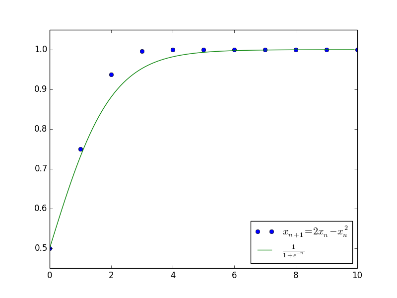
The question now is: since the solution of the differential equation can serve as a well-behaved approximate solution, is it possible to further add correction terms based on the differential equation solution to improve accuracy?

General Format

We introduce a parameter q and consider a more general difference equation: \label{yibanchafenfangcheng} x_{n+q}-x_n = q f(x_n) When q=1, it is exactly the difference equation [chafenfangcheng] we are considering, and when q \to 0, it becomes the differential equation: \frac{dx}{dn}=f(x) Note that since we have introduced q, the specific form of x_n depends on q. In other words, x_n is actually a function of q, which we write explicitly as x_{n,q}, namely: \label{yibanchafenfangcheng2} x_{n+q,q}-x_{n,q}=qf(x_{n,q}) Our ultimate interest is x_n \equiv x_{n,1}. To solve this equation step-by-step, we imagine that x_{n,q} can be expanded as a power series in q: x_{n,q}=\sum_{k=0}^{\infty}a^{(k)}_n q^k where a_n^{(k)} = \frac{1}{k!}\left.\frac{\partial^k x_{n,q}}{\partial q^k}\right|_{q=0},\quad k=0,1,2,\dots The problem now is how to find each a_n^{(k)}.

Step-by-step Expansion

Taking the total derivative with respect to q on both sides of equation [yibanchafenfangcheng2], we get: \label{qiudao} \frac{\partial x_{n+q,q}}{\partial n}+\frac{\partial x_{n+q,q}}{\partial q}-\frac{\partial x_{n,q}}{\partial q}=f(x_{n,q})+q\frac{\partial f}{\partial x_{n,q}}\frac{\partial x_{n,q}}{\partial q} It should be noted that when we write \frac{\partial x_{n+q,q}}{\partial q} by default, we only differentiate with respect to the second variable q, and not with respect to the q in the first variable n+q. Now setting q=0, we have: \label{qiudao-q-0} \frac{\partial x_{n,0}}{\partial n}=f(x_{n,0}) This is exactly the differential equation [weifenfangcheng] used as the first approximation.

Next, differentiating [qiudao] with respect to q again: \label{qiudao2} \begin{aligned} &\frac{\partial^2 x_{n+q,q}}{\partial n^2}+2\frac{\partial^2 x_{n+q,q}}{\partial n \partial q}+\frac{\partial^2 x_{n+q,q}}{\partial q^2}-\frac{\partial^2 x_{n,q}}{\partial q^2}\\ =&2\frac{\partial f}{\partial x_{n,q}}\frac{\partial x_{n,q}}{\partial q}+q\frac{\partial^2 f}{\partial x_{n,q}^2}\left(\frac{\partial x_{n,q}}{\partial q}\right)^2+q\frac{\partial f}{\partial x_{n,q}}\frac{\partial^2 x_{n,q}}{\partial q^2} \end{aligned} Letting q=0, we obtain: \label{qiudao2-q-0} \frac{\partial^2 x_{n,0}}{\partial n^2}+2\frac{\partial}{\partial n}\left(\frac{\partial x_{n,0}}{\partial q}\right)=2\frac{\partial f}{\partial x_{n,0}}\frac{\partial x_{n,0}}{\partial q} The term \frac{\partial^2 x_{n,0}}{\partial n^2} can be calculated by substituting the x_{n,0} obtained in the previous step. Therefore, this is a first-order linear differential equation for \frac{\partial x_{n,0}}{\partial q}, which is also solvable. This process can be continued to gradually improve accuracy. The subsequent forms are too tedious to write out and can be handled using Mathematica.

Discrete Logistic Growth Model

A concrete example will make the process clearer. Reconsidering the logistic growth model [zuzhizengzhang], after introducing the parameter q, the equation is written as: x_{n+q,q}-x_{n,q}=q\alpha x_{n,q}-q\beta x_{n,q}^2 Here f(x)=\alpha x - \beta x^2, and the corresponding equation [qiudao-q-0] is: \frac{\partial x_{n,0}}{\partial n}=\alpha x_{n,0}-\beta x_{n,0}^2 The solution has already been found: x_{n,0}=\frac{\alpha}{\beta+c e^{-\alpha n}} This is the zero-order approximation. Correspondingly, the equation [qiudao2-q-0] is: \frac{\partial^2 x_{n,0}}{\partial n^2}+2\frac{\partial}{\partial n}\left(\frac{\partial x_{n,0}}{\partial q}\right)=2(\alpha-2\beta x_{n,0})\frac{\partial x_{n,0}}{\partial q} The solution is (obtained using Mathematica and simplified manually, setting \frac{\partial x_{0,0}}{\partial q}=0): \frac{\partial x_{n,0}}{\partial q}=\left(\frac{\alpha}{\beta+ce^{-\alpha n}}\right)^2\left(\frac{1}{2}\alpha n-\ln \frac{\beta+c}{\beta+ce^{-\alpha n}}\right)ce^{-\alpha n} Therefore, we have: x_{n,q}\approx \frac{\alpha}{\beta+c e^{-\alpha n}}+q\left(\frac{\alpha}{\beta+ce^{-\alpha n}}\right)^2\left(\frac{1}{2}\alpha n-\ln \frac{\beta+c}{\beta+ce^{-\alpha n}}\right)ce^{-\alpha n} And: x_n\equiv x_{n,1}\approx \frac{\alpha}{\beta+c e^{-\alpha n}}+\left(\frac{\alpha}{\beta+ce^{-\alpha n}}\right)^2\left(\frac{1}{2}\alpha n-\ln \frac{\beta+c}{\beta+ce^{-\alpha n}}\right)ce^{-\alpha n} This is its first-order approximation. The figure below shows a comparison between the zero-order and first-order approximate solutions and the exact values when \alpha=\beta=1 and c=1 (i.e., x_0=\frac{1}{2}). It can be seen that compared to the zero-order approximation, the first-order approximation almost coincides with the exact values.

This example also illustrates the characteristics of the perturbation method. Although it can be continued and each step is integrable, the integrals may become too complex to be useful.

A Note

Theoretically, this perturbation scheme can find approximate solutions for any first-order difference equation. Of course, whether it is truly practical in real applications depends on the specific problem.

First, if the solution to the zero-order differential equation (which is nonlinear) is too complex, it will be difficult to proceed with this method. Second, although each step only generates a theoretically solvable first-order non-homogeneous linear differential equation, solving this equation is not always simple; often, the time and effort required for each additional step are doubled.

Finally, it should be noted that the format for introducing parameters is not limited to [yibanchafenfangcheng2]. It can be simplified according to the specific problem. For example, in the article "Implicit Function Solution of a Nonlinear Difference Equation": x_{n+1}=x_n+3+\frac{3}{x_n}+\frac{1}{x_n^2},\,x_1=1 The parameter can be introduced as: x_{n+q,q}=x_{n,q}+3+\frac{3q}{x_{n,q}}+\frac{q^2}{x_{n,q}^2},\,x_1=1 This will yield the same asymptotic solution as in that article. This reflects the essence of the perturbation method, which is to identify the order of each term through the parameter q, thereby allowing for step-by-step approximation. What is chosen as the order, much like what is chosen as the parameter, is largely a matter of choice.

When reposting, please include the original link: https://kexue.fm/archives/3889

For more details on reposting, please refer to: Scientific Space FAQ