Path Integral Series: 3. Path Integral

From Point Probability to Path Probability

In the study of random walks in the previous chapter, we concluded that the probability density of starting from x_0 and reaching x_n after time t is: \frac{1}{\sqrt{2\pi \alpha t}}\exp\left(-\frac{(x_n-x_0)^2}{2\alpha t}\right). \tag{22} This is the probability from one point at one moment to another point at another moment. In mathematics, we call this the propagator of the diffusion equation (21), or the Green’s function.

Now, divide the time T into n equal parts, each of length \Delta t = \frac{T}{n}. At time i\Delta t, the particle’s position is x_k. The probability density for the particle to go from x_k to x_{k+1} is: \frac{1}{\sqrt{2\pi \alpha \Delta t}}\exp\left(-\frac{(x_{k+1}-x_k)^2}{2\alpha \Delta t}\right), \tag{23} so the probability density for the particle to pass through x_1, x_2, \dots, x_{n-1}, x_n in sequence is: \left(\frac{1}{\sqrt{2\pi \alpha \Delta t}}\right)^n \exp\left(-\frac{(x_1-x_0)^2+(x_2-x_1)^2+\dots+(x_n-x_{n-1})^2}{2\alpha \Delta t}\right). \tag{24} Temporarily omitting the preceding factors and taking the limit \Delta t \to 0, we consider that these points x_0, x_1, x_2, \dots, x_{n-1}, x_n define a path x(t) from (x_0, 0) to (x_n, T), and: \frac{(x_1-x_0)^2+(x_2-x_1)^2+\dots+(x_n-x_{n-1})^2}{2\alpha \Delta t} = \frac{1}{2\alpha}\sum_{k=0}^{n-1} \left(\frac{x_{k+1}-x_k}{\Delta t}\right)^2 \Delta t, \tag{25} As \Delta t \to 0, we consider \frac{x_{k+1}-x_k}{\Delta t} to be equal to the derivative \dot{x}(t_k) of x(t) at t_k. Thus, the above expression is precisely the discrete expression of the integral \frac{1}{2\alpha}\int \dot{x}^2 dt. In summary, we obtain that the probability of a particle traveling along the path x=x(t) is proportional to: P[x(t)] = \exp\left(-\frac{1}{2\alpha} \int \dot{x}^2 dt\right). \tag{26} This gives the probability of the particle passing through path x(t), which is a functional of x(t). This is the path probability distribution for Brownian motion. If \alpha=1, it is called standard Brownian motion.

Note:

If W_t is a stochastic process satisfying the following conditions, it is called a Brownian motion:

1. W_0 = 0;

2. \{W_t, t \geq 0\} is a process with stationary independent increments;

3. \forall 0 \leq s \leq t, W_t - W_s \sim N(0, \sigma^2(t-s)).

When \sigma=1, it is called standard Brownian motion.

Summing Over Paths

We have obtained the expression for the probability P[x(t)] of a specific path. The probability of going from (x_0, 0) to (x_n, T) should be the sum of the probabilities of all paths from (x_0, 0) to (x_n, T). In other words, we must traverse and sum over all paths between the two points.

Traversing is achieved by discretizing the path. As shown in Figure 1, we still divide the time T. For every path, we can approximate it with the polyline x_0, x_1, x_2, \dots, x_{n-2}, x_{n-1}, x_n. Therefore, to traverse all paths x(t), we only need to traverse all x_1, x_2, \dots, x_{n-2}, x_{n-1} (imagine "toggling" each point x_1, x_2, \dots, x_{n-1} up and down).

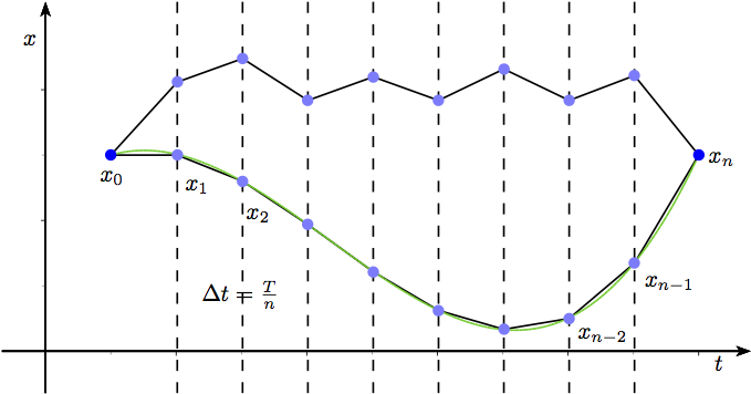
Discretizing a path and then traversing

If we use P(x_0, 0; x_n, T) to represent the probability of reaching (x_n, T) from (x_0, 0), then (for brevity, we omit the constant factors, which we can restore in practical problems; for now, we want to clarify the concept): \begin{aligned} &P(x_0, 0; x_n, T) \\ =& \lim_{n\to\infty} \int_{-\infty}^{\infty} \exp\left(-\frac{1}{2\alpha}\sum_{k=0}^{n-1} \left(\frac{x_{k+1}-x_k}{\Delta t}\right)^2 \Delta t\right) dx_1 dx_2 \dots dx_{n-2} dx_{n-1} \end{aligned}, \tag{27} The integration is performed n-1 times, and then the limit n \to \infty is taken. We denote the above expression concisely as: P(x_0, 0; x_n, T) = \int_{x_0}^{x_n} P[x(t)] \mathscr{D}x(t) = \int_{x_0}^{x_n} \exp\left(-\frac{1}{2\alpha} \int_0^T \dot{x}^2 dt\right) \mathscr{D}x(t), \tag{28} This is called the path integral (or functional integral) of the functional P[x(t)], which is an infinite-dimensional integral.

Path Integral of Parabolic Equations

This section aims to convert the parabolic equation (19) into a path integral representation. From equation (27), we know that the key to constructing a path integral is to find the propagator (Green’s function) within an infinitesimal time interval.

First, consider the case where V=V(x), i.e., independent of time. Let H = \frac{\alpha^2}{2}\frac{\partial^2}{\partial x^2} + V, and rewrite equation (19) as: \alpha \frac{\partial \phi}{\partial t} = H\phi, \tag{29} Since H is independent of t, the solution to the above equation can be formally written as: \phi(x, t) = \exp\left(\frac{1}{\alpha} t H\right) \phi(x, 0) = \exp\left[\frac{1}{\alpha} t \left(\frac{\alpha^2}{2}\frac{\partial^2}{\partial x^2} + V(x)\right)\right] \phi(x, 0). \tag{30}

The above formula is an exact solution, where \exp\left(\frac{1}{\alpha} t H\right) should be understood as an operator series: \exp\left(\frac{1}{\alpha} t H\right) = \sum_{k=0}^{\infty} \frac{1}{k!} \frac{t^k}{\alpha^k} H^k. \tag{31}

Now we are only concerned with the result for an infinitesimal interval, i.e., taking t = \epsilon \to 0: \phi(x, \epsilon) = \exp\left(\frac{\alpha}{2} \epsilon \frac{\partial^2}{\partial x^2} + \frac{1}{\alpha} \epsilon V(x)\right) \phi(x, 0), \tag{32} Note that \frac{\partial^2}{\partial x^2} and V(x) are generally non-commutative, so in general: \exp\left(\frac{\alpha}{2} \epsilon \frac{\partial^2}{\partial x^2} + \frac{1}{\alpha} \epsilon V(x)\right) \neq \exp\left(\frac{\alpha}{2} \epsilon \frac{\partial^2}{\partial x^2}\right) \exp\left(\frac{1}{\alpha} \epsilon V(x)\right), \tag{33} However, in the case of a first-order approximation, the two are equal (that is, the difference between them is a second-order infinitesimal). So we have: \phi(x, \epsilon) = \exp\left(\frac{1}{\alpha} \epsilon V(x)\right) \exp\left(\frac{\alpha}{2} \epsilon \frac{\partial^2}{\partial x^2}\right) \phi(x, 0), \tag{34} Notice that: \hat{\phi}(x, \epsilon) = \exp\left(\frac{\alpha}{2} \epsilon \frac{\partial^2}{\partial x^2}\right) \phi(x, 0), \tag{35} is exactly the formal solution to the diffusion equation \frac{\partial \hat{\phi}}{\partial t} = \frac{\alpha}{2} \frac{\partial^2 \hat{\phi}}{\partial x^2}. From mathematical physics tutorials, we have already obtained its general solution: \hat{\phi}(x, \epsilon) = \int_{-\infty}^{\infty} \frac{1}{\sqrt{2\pi \alpha \epsilon}} \exp\left(-\frac{1}{\alpha} \frac{(x-x_0)^2}{2\epsilon}\right) \phi(x_0, 0) dx_0, \tag{36} So equation (34) equals: \begin{aligned} \phi(x, \epsilon) &= \exp\left(\frac{1}{\alpha} \epsilon V(x)\right) \int_{-\infty}^{\infty} \frac{1}{\sqrt{2\pi \alpha \epsilon}} \exp\left(-\frac{1}{\alpha} \frac{(x-x_0)^2}{2\epsilon}\right) \phi(x_0, 0) dx_0 \\ &= \frac{1}{\sqrt{2\pi \alpha \epsilon}} \int_{-\infty}^{\infty} \exp\left[-\frac{1}{\alpha} \left(\frac{1}{2} \frac{(x-x_0)^2}{\epsilon^2} - V(x)\right) \epsilon\right] \phi(x_0, 0) dx_0 \end{aligned}, \tag{37} Since the above equation is for an infinitesimal time interval, \frac{x-x_0}{\epsilon} can be considered as the first derivative \dot{x}. Therefore, the Green’s function for an infinitesimal time is (omitting the preceding factor): \exp\left[-\frac{1}{\alpha} \left(\frac{1}{2} \dot{x}^2 - V(x)\right) \epsilon\right], \tag{38} Thus, we can successively find: \begin{aligned} &K(x_0, 0; x_n, T) \\ &= \lim_{n\to\infty} \int_{-\infty}^{\infty} \exp\left\{-\frac{1}{2\alpha} \sum_{k=0}^{n-1} \left[\left(\frac{x_{k+1}-x_k}{\Delta t}\right)^2 - V(x_k)\right] \Delta t\right\} dx_1 \dots dx_{n-1} \end{aligned}, \tag{39} Since \phi is not a probability in the true sense, K is used here to represent the propagator of \phi. The above equation implies that the probability functional for passing through a certain path x(t) is: K[x(t)] = \exp\left[-\frac{1}{\alpha} \int_{t_a}^{t_b} \left(\frac{1}{2} \dot{x}^2 - V(x)\right) dt\right], \tag{40} In this way, the probability from point (x_a, t_a) to point (x_b, t_b) can be expressed as a path integral between the two points: \begin{aligned} P(x_b, t_b; x_a, t_a) &= \int_{x_a}^{x_b} P[x(t)] \mathscr{D}x(t) \\ &= \int_{x_a}^{x_b} \exp\left[-\frac{1}{\alpha} \int_{t_a}^{t_b} \left(\frac{1}{2} \dot{x}^2 - V(x)\right) dt\right] \mathscr{D}x(t) \end{aligned}. \tag{41} The above derivation is based on the special case where V is independent of time t, but with simple modifications, it can be used for time-dependent cases, which will not be repeated here.

From Path Integral to Partial Differential Equations

Starting from the path functional in (40) and performing the path integral, one can conversely derive the partial differential equation (19). The specific process can be found in "Quantum Mechanics and Path Integrals"; it will not be repeated here. Since they can be derived from each other, it means the two are equivalent. Given a partial differential equation in the form of (19), the corresponding path functional (40) can be written immediately, and vice versa.

Some Examples

The path integral is conceptually quite simple, but the calculation is very complex. There are very few solutions that can be calculated exactly; most of the time, approximations are used. This section provides some results without proof. These results come from works such as "Quantum Mechanics and Path Integrals" and "Statistical Mechanics" by the physicist Feynman. This is merely to show readers that effective calculation schemes already exist for many path integral problems.