Modeling a Year Late: Revisiting Shredded Paper Reconstruction

Greedy Algorithm

In the matching of shredded paper, we mainly used the greedy algorithm. The main steps involve manually selecting a starting fragment as the origin, then comparing the rightmost edge vector of this fragment’s pixel matrix with the leftmost edge vectors of other fragments, selecting the fragment with the highest matching degree. Then, using the newly matched fragment as the new starting point, we perform optimal matching for the remaining fragments, and so on.

The greedy algorithm is an algorithm that seeks local optima in hopes of reaching a global optimum. It is easy to program and highly efficient. However, because it only seeks local optima at each step, we cannot predict whether the result will be globally optimal. In shredded paper reconstruction, this algorithm may lead to two anomalies:

1. Different starting points result in different stitching outcomes.

2. When edge information is scarce, matching errors occur frequently.

To (partially) avoid the shortcomings of the greedy algorithm, we improved it with manual intervention. Testing showed that Attachments 1 and 2 do not require additional manual intervention; therefore, our manual intervention was designed only for Attachments 3 and 4. The details of the improvement will be described in the section on Manual Intervention.

Matching Degree

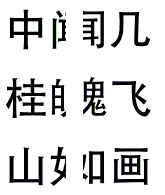
As shown in the figure above, generally speaking, considering image continuity, the edge pixels of two adjacent fragments should be similar or even identical. This naturally suggests that the matching metric for two edges is the distance between two vectors: d^2=|\boldsymbol{x}-\boldsymbol{y}|^2=\sum_{i=1}^{n}(x_i-y_i)^2

If the distance between two edge vectors is 0, we can say with certainty that these two fragments match. But when the distance is large, how certain can we be that they do not match? We know that general images possess not only continuity but also gradual transitions. For a general image, adjacent column vectors can be considered to transition linearly. Thus, the matching degree seems better measured by "linear correlation." The formula for the linear correlation coefficient [3] is: \rho_{X,Y}={\mathrm{cov}(X,Y) \over \sigma_X \sigma_Y} ={E[(X-\mu_X)(Y-\mu_Y)] \over \sigma_X\sigma_Y}

The calculation formula for the linear correlation coefficient is much more complex than the distance formula. We tested both metrics on the same set of fragments. After testing fragments with different contents, we found that, overall, using the linear correlation coefficient performed better than the distance formula. However, the advantage of the correlation coefficient was mainly evident in the reconstruction of photographic shredded paper (fragments generated by our team for testing), while for the text-based fragments provided officially, there was no significant difference. Ultimately, for simplicity, we chose vector distance as our matching metric.

Manual Intervention

This section is designed for Attachments 3 and 4. To facilitate manual intervention, we labeled the filename on each fragment during the stitching process without modifying the original fragment files.

First, if the code for Attachments 1 and 2 is applied directly to Attachment 3, the following effect (partial) occurs:

All fragments are stitched into a long strip, containing both correctly stitched parts and many errors. From another perspective, the fragments are currently stitched into a pile of (about 20–30) larger fragment blocks. This means we can fix the correctly stitched parts and then stitch these blocks together. This reduces the task from over 200 fragments to about 20 blocks, significantly reducing the workload. This requires a person to identify correctly stitched parts from the image and record them in the code. In fact, this is equivalent to a manual clustering process. (We did not use an automated clustering algorithm here; the reasons will be explained in the difficulty analysis.)

In addition, we introduced "manual exclusion." When two distances are very close, the greedy algorithm may produce a matching error. However, we must recognize that this does not happen frequently. When edge information is sufficient, or after fragments have been clustered, matching errors are low-probability events. Therefore, if we observe a matching error, we can manually exclude that specific match, forcing the program to choose the next best option from the remaining candidates. We believe that after a few (very few) exclusions, the program will automatically match the correct fragments.

Once further correct stitching information is obtained, it can be added to the code, followed by more exclusions and manual stitching. Repeating this process allows the reconstruction to be completed within an "acceptable" timeframe.

Attachments 1 and 2

We use Attachment 1 as an example. The stitching code for Attachment 1 is in the appendix. First, specify an arbitrary starting image (the m value in the code), then judge the correct starting image (008.bmp) based on the result, modify the m value, and run it again. Tests show no extra manual intervention is needed. The final sequence for Attachment 1 is:

[8, 14, 12, 15, 3, 10, 2, 16, 1, 4, 5, 9, 13, 18, 11, 7, 17, 0, 6]

The process for Attachment 2 is basically the same, resulting in:

[3, 6, 2, 7, 15, 18, 11, 0, 5, 1, 9, 13, 10, 8, 12, 14, 17, 16, 4]

Attachments 3 and 4

The code for Attachment 3 was modified from Attachment 1, mainly adding filename labeling, manual stitching, and manual exclusion. Running the code directly yields a sequence (partial):

[14, 128, 3, 159, 82, 199, 7, 208, 29, 64, 111, 201, 5, 92, 180, 48, 37, 75, 38, 148, ...]

Observation shows that [14, 128, 3, 159, 82, 199] is correct, [7, 208] is correct, [29, 64, 111, 201, 5, 92, 180, 48, 37, 75] is correct, etc. Thus, we add the following lines under known=[[] for i in range(0,num)]:

known[14] = [128, 3, 159, 82, 199]
known[7] = [208]
known[29] = [64, 111, 201, 5, 92, 180, 48, 37, 75]
...

Furthermore, it is observed that matching 7 after 199 is wrong, matching 29 after 208 is wrong, and 75 cannot match 38. Thus, under impossible=[[] for i in range(0,num)], we add:

impossible[199] = [7]
impossible[208] = [29]
impossible[75] = [38]
...

After modifications, rerun the script to get a new sequence. Add new correct segments and easily identifiable manual matches to known, and add obvious errors to impossible. Repeat this operation. Within about two hours, the stitching for each row of Attachment 3 can be completed. That is, stitch each row first, generate images for each row, and then perform vertical stitching.

The same approach can be used to complete Attachment 4.

Clustering is hard to make effective

Although clustering can reduce some workload, its actual effect is very small. In our code, even if we manually find 19 fragments belonging to the same row and use the algorithm for automatic stitching, the result is still not ideal due to insufficient edge information, which is unavoidable.

Secondly, clustering has too many limitations. The competition fragments are cut from articles, which have obvious patterns (same font size, same line spacing, etc.), allowing for preliminary clustering. However, for general fragments like photos, there is no similar clustering method. Therefore, clustering is hard to make effective and only provides constant-level optimization in this problem.

Vertical information is hard to utilize

After completing the horizontal stitching for each row of Attachment 3, our team obtained 11 horizontal strips. However, even using these 11 strips as raw materials, automatic stitching still produced many errors and could not be completed automatically. This means that even after completing the horizontal stitching, the information provided by vertical edges is still very scarce. If one wanted to use vertical information while dealing with over 200 small fragments at the start, it would be nearly impossible. Thus, it can be said that during the stitching process, only horizontal information is usable, which increases the difficulty.

Lessons from the past

Shredded paper reconstruction is inherently a very difficult problem. The DARPA Shredder Challenge mentioned at the beginning was won by a team that took over a month to complete the task. [4] Although the difficulties of the two problems are not directly comparable, this reflects the overall difficulty of shredded paper reconstruction. Therefore, the two-plus hours spent on Attachment 3 in this paper should be considered within a reasonable timeframe.

Code for Attachments 1 and 2

import os
import numpy
from PIL import Image

# Get current directory list
images = os.listdir(os.getcwd())
images.remove('c.py') # Script filename
num = len(images) # Number of images

hang = Image.open(images[0]).size[1] # Image height
lie = Image.open(images[0]).size[0] # Image width
bianyuan = numpy.zeros((hang, 2*num)) # Matrix to store edge information

# Open images, get edge values
for i in range(0, num):
    img = Image.open(images[i])
    bianyuan[:, 2*i+1] = numpy.array(img)[:, 0] # Left edge info in odd columns
    bianyuan[:, 2*i] = numpy.array(img)[:, lie-1] # Right edge info in even columns
# Edge values acquired

i = 0; m = 31 # m is the starting point
xulie = [m] # Store stitching sequence
temp = [k for k in range(0, num)]
while i < num-1:
    m1 = temp[m]
    temp.remove(temp[m])
    bijiao = numpy.zeros(len(temp)) # Comparison matrix
    for j in range(0, len(temp)):
        # Compare each right edge with all left edges
        bijiao[j] = numpy.sum((bianyuan[:, 2*m1] - bianyuan[:, 2*temp[j]+1])**2)
    m = numpy.argmin(bijiao) # Minimum difference means highest match
    xulie.append(temp[m])
    i = i + 1
print(xulie) # Output sequence

comb_img = Image.new("RGBA", (lie*num, hang), (255, 0, 0)) # New image for synthesis
j = 0
for i in xulie:
    img = Image.open(images[i])
    region = img.crop((0, 0, lie, hang))
    comb_img.paste(region, (lie*j, 0, lie*(j+1), hang))
    j = j + 1
comb_img.show()

Code for Attachments 3 and 4

import os
import numpy
from PIL import Image
from PIL import ImageDraw
from PIL import ImageFont

# Get current directory list
images = os.listdir(os.getcwd())
images.remove('c.py')
num = len(images) # Number of images

hang = Image.open(images[0]).size[1] # Image height
lie = Image.open(images[0]).size[0] # Image width
bianyuan = numpy.zeros((hang, 2*num)) # Matrix to store edge information

# Open images, get edge values
for i in range(0, num):
    img = Image.open(images[i])
    bianyuan[:, 2*i+1] = numpy.array(img)[:, 0] # Left edge info in odd columns
    bianyuan[:, 2*i] = numpy.array(img)[:, lie-1] # Right edge info in even columns
# Edge values acquired

known = [[] for i in range(0, num)] # Known stitching
impossible = [[] for i in range(0, num)] # Excluded stitching

i = 0; m = 14 # m is the starting point
m1 = m
xulie = [m] # Store stitching sequence
temp = [k for k in range(0, num)]
temp.remove(m1)

for kn in known:
    for knn in kn:
        try:
            temp.remove(knn) # Remove known cases
        except: pass

while i < num-1:
    if len(known[m1]) != 0:
        m2 = 0
        for kn in known[m1]:
            xulie.append(kn)
            m2 = kn
            i = i + 1
        m1 = m2
    else:
        temp1 = temp[:]
        for imp in impossible[m1]:
            try:
                temp.remove(imp)
            except: pass
        bijiao = numpy.zeros(len(temp)) # Comparison matrix
        for j in range(0, len(temp)):
            # Compare each right edge with all left edges
            bijiao[j] = numpy.sum((bianyuan[:, 2*m1] - bianyuan[:, 2*temp[j]+1])**2)
        m = numpy.argmin(bijiao) # Minimum difference means highest match
        xulie.append(temp[m])
        i = i + 1
        m1 = temp[m]
        temp = temp1[:]
        temp.remove(m1)
print(xulie) # Output sequence

# Add watermark
myfont = ImageFont.truetype("arial.ttf", 36) # Font and size

comb_img = Image.new("RGBA", (lie*num, hang), (255, 0, 0)) # New image for synthesis
j = 0
for i in xulie:
    img = Image.open(images[i])
    d = ImageDraw.Draw(img) # Draw watermark
    d.ink = 150 # Watermark color
    d.text((0, 0), str(i), font=myfont) # Add filename as watermark
    region = img.crop((0, 0, lie, hang))
    comb_img.paste(region, (lie*j, 0, lie*(j+1), hang))
    j = j + 1
comb_img.show()

Final Modification Results (Attachment 3)

known = [[] for i in range(0, num)] # Known stitching
known[14] = [128, 3, 159, 82, 199, 135, 12, 73, 160, 203, 169, 134, 39, 31, 51, 107, 115, 176, 94]
known[94] = [34, 84, 183, 90, 47, 121, 42, 124, 144, 77, 112, 149, 97, 136, 164, 127, 58, 43, 7]
known[7] = [208, 138, 158, 126, 68, 175, 45, 174, 0, 137, 53, 56, 93, 153, 70, 166, 32, 196, 38]
known[38] = [148, 46, 161, 24, 35, 81, 189, 122, 103, 130, 193, 88, 167, 25, 8, 9, 105, 74, 168]
known[168] = [100, 76, 62, 142, 30, 41, 23, 147, 191, 50, 179, 120, 86, 195, 26, 1, 87, 18, 29]
known[29] = [64, 111, 201, 5, 92, 180, 48, 37, 75, 55, 44, 206, 10, 104, 98, 172, 171, 59, 61]
known[61] = [19, 78, 67, 69, 99, 162, 96, 131, 79, 63, 116, 163, 72, 6, 177, 20, 52, 36, 49]
known[49] = [54, 65, 143, 186, 2, 57, 192, 178, 118, 190, 95, 11, 22, 129, 28, 91, 188, 141, 125]
known[125] = [13, 182, 109, 197, 16, 184, 110, 187, 66, 106, 150, 21, 173, 157, 181, 204, 139, 145, 89]
known[89] = [146, 102, 154, 114, 40, 151, 207, 155, 140, 185, 108, 117, 4, 101, 113, 194, 119, 123]
known[71] = [156, 83, 132, 200, 17, 80, 33, 202, 198, 15, 133, 170, 205, 85, 152, 165, 27, 60]

impossible = [[] for i in range(0, num)] # Excluded stitching
impossible[199] = [7, 29, 38, 49, 61, 62, 67, 71, 80, 89, 94, 125]
impossible[1] = [146, 129, 102, 134]
impossible[79] = [71, 146, 89, 94]
impossible[123] = [94, 125]
impossible[176] = [7]
impossible[13] = [135, 94]
impossible[160] = [143, 168, 146, 25, 94, 7, 29, 38, 49]
impossible[95] = [168, 129]
impossible[124] = [136, 8, 46, 138, 129]
impossible[58] = [161, 46, 182, 83]
impossible[46] = [9]
impossible[97] = [144]
impossible[25] = [168]

Final Modification Results (Attachment 4)

known = [[] for i in range(0, num)] # Known stitching
known[20] = [41, 108, 116, 136, 73, 36, 207, 135, 15, 76, 43, 199, 45, 173, 79, 161, 179, 143, 86]
known[86] = [51, 107, 29, 40, 158, 186, 98, 24, 117, 150, 5, 59, 58, 92, 30, 37, 46, 127, 201]
known[201] = [148, 170, 196, 198, 94, 113, 164, 78, 103, 91, 80, 101, 26, 100, 6, 17, 28, 146, 208]
known[208] = [21, 7, 49, 61, 119, 33, 142, 168, 62, 169, 54, 192, 133, 118, 189, 162, 197, 112, 171]
known[171] = [42, 66, 205, 10, 157, 74, 145, 83, 134, 55, 18, 56, 35, 16, 9, 183, 152, 44, 132]
known[132] = [181, 95, 69, 167, 163, 166, 188, 111, 144, 206, 3, 130, 34, 13, 110, 25, 27, 178, 70]
known[70] = [84, 60, 14, 68, 174, 137, 195, 8, 47, 172, 156, 96, 23, 99, 122, 90, 185, 109, 81]
known[81] = [77, 128, 200, 131, 52, 125, 140, 193, 87, 89, 48, 72, 12, 177, 124, 0, 102, 115]
known[19] = [194, 93, 141, 88, 121, 126, 105, 155, 114, 176, 182, 151, 22, 57, 202, 71, 165, 82]
known[191] = [75, 11, 154, 190, 184, 2, 104, 180, 64, 106, 4, 149, 32, 204, 65, 39, 67, 147]
known[159] = [139, 1, 129, 63, 138, 153, 53, 38, 123, 120, 175, 85, 50, 160, 187, 97, 203, 31]

impossible = [[] for i in range(0, num)] # Excluded stitching
impossible[16] = [30, 178, 195, 150, 186, 2, 19, 70, 81, 132]
impossible[122] = [109, 197, 32]
impossible[137] = [32]
impossible[204] = [4, 54]
impossible[22] = [82]
impossible[12] = [120, 149, 159]
impossible[175] = [24, 1]
impossible[158] = [30, 195]
impossible[190] = [54, 4]
impossible[144] = [197, 32, 178, 195]
impossible[121] = [167, 169]
impossible[150] = [130]
impossible[176] = [88]
impossible[141] = [182, 70, 81]
impossible[124] = [3]
impossible[138] = [102, 0]
impossible[65] = [169, 184, 2]
impossible[165] = [9]
impossible[119] = [32, 195, 70]
impossible[27] = [177, 195]
impossible[169] = [4]
impossible[62] = [126]
impossible[193] = [85, 177]
impossible[162] = [70]
impossible[31] = [149]
impossible[184] = [202]
impossible[85] = [102]
impossible[57] = [88]

Please include the original address when reprinting: https://kexue.fm/archives/3134

For more details on reprinting, please refer to: Scientific Space FAQ