Infinite Decomposition of Force and the Green's Function Method

Infinite Decomposition of Force

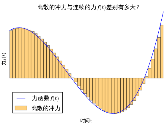
Of course, the above was just a "whimsical" thought from my childhood; readers need not take it too seriously. However, what is the connection between this question and this article? When we study vibration problems, we often encounter forced vibration under the action of a variable force. Suppose the variable force is a function of time, such as f(t). Even if the specific form of f(t) is known, the motion after adding the external force is not necessarily easy to solve due to the nonlinearity of f. However, if a variable force can be segmented into constant forces (impulses) over infinite infinitesimal time intervals, then we can discuss the motion we want to study segment by segment. Generally speaking, problems involving constant forces are easier than those involving variable forces. If we discretize a variable force and then take the limit, is the resulting motion the same as the motion under the original variable force? This shares a similar idea with the question at the beginning of the article—is the limit of the discrete equivalent to the continuous itself?

Surprisingly, in common physical systems, the practice of segmenting a force into constant forces within infinite small intervals leads to the correct answer. Moreover, this happens to be the Green’s function method for linear ordinary differential equations. Let us analyze this approach below.

First-Order Ordinary Differential Equations

As a simple first example, let us solve: \frac{dx(t)}{dt}+x(t)=f(t) This is, of course, a simple ordinary differential equation for which the method of variation of constants is available. For now, let us forget that method and re-understand this equation. When f(t) \equiv 0, the equation is easy to solve; when f(t) is a non-zero constant, solving it is also not difficult—one simply adds a constant to the original solution. But when f(t) is a general function, the solution becomes complicated. Suppose we already know the state x(t) at time t; let us try to derive the state x(t+\varepsilon) at time t+\varepsilon. Here, \varepsilon is a very small time interval, so small that f(t) barely changes during this period. Thus, within the interval [t, t+\varepsilon], we treat the external force as a constant f(t). In this case, we have: \frac{d x(t+s)}{ds}+x(t+s)=f(t),\quad 0\leq s\leq \varepsilon The general solution to this equation is: x(t+s)=C e^{-s}+f(t) (Note: The original text used C e^{-t-s}, which is equivalent by adjusting the constant C). At s=0, we have x(t)=C+f(t), so C=x(t)-f(t). Thus we obtain: x(t+s)=[x(t)-f(t)]e^{-s}+f(t) Consequently: \begin{aligned}x(t+\varepsilon)=&[x(t)-f(t)]e^{-\varepsilon}+f(t)\\ =&x(t)e^{-\varepsilon}+(1-e^{-\varepsilon})f(t)\\ =&x(t)(1-\varepsilon)+\varepsilon f(t)\end{aligned} Of course, this step is trivial; we could have obtained this result directly from the original differential equation because we only care about the first-order infinitesimal: \frac{x(t+\varepsilon)-x(t)}{\varepsilon}\approx\frac{dx(t)}{dt}=-x(t)+f(t) Simple rearrangement gives x(t+\varepsilon)=x(t)(1-\varepsilon)+f(t)\varepsilon, which is equivalent to the previous expression. However, through the above discourse, we can endow our method with intuitive physical meaning, which is why we are willing to go through slightly longer steps.

Note the characteristics of this solution. From the state x(t) at time t, we obtained the state at t+\varepsilon. By iterating this n times, we can obtain the state at time t+n\varepsilon: \begin{aligned}x(t+n\varepsilon)=&x(t+(n-1)\varepsilon)e^{-\varepsilon}+f(t+(n-1)\varepsilon)\varepsilon\\ =&[x(t+(n-2)\varepsilon)e^{-\varepsilon}+f(t+(n-2)\varepsilon)\varepsilon] e^{-\varepsilon}+f(t+(n-1)\varepsilon)\varepsilon\\ =&x(t+(n-2)\varepsilon)e^{-2\varepsilon}+ [e^{-\varepsilon}f(t+(n-2)\varepsilon)+f(t+(n-1)\varepsilon)]\varepsilon\\ =&\dots\\ =&x(t)e^{-n\varepsilon}+\varepsilon\sum_{i=1}^n e^{-(i-1)\varepsilon}f(t+n\varepsilon-i\varepsilon)\end{aligned} Fixing n\varepsilon=\tau and letting n\to\infty, we get: \begin{aligned}x(t+\tau)=&x(t)e^{-\tau}+\int_0^\tau e^{-s}f(t+\tau-s)ds\\ =&x(t)e^{-\tau}-\int_t^{t+\tau} e^{-t-\tau+s}f(s)ds\end{aligned} Thus we have obtained the (exact) solution at time t+\tau. By substituting any known initial state, we can find the state at any time. Here, G(t,s)=e^{-t+s} is called the Green’s function of the system, with which we can obtain x(t) from x(s).

Second-Order Ordinary Differential Equations

The case of first-order equations is too trivial, to the point where one might think it lacks value. Now, using the same idea, let us provide the Green’s function solution for: \frac{d^2 x(t)}{dt^2}+x(t)=f(t) Unlike the first-order case, due to the increase in order, the derivation process involves matrix and vector operations. This equation is equivalent to the system: \frac{d}{dt}\begin{pmatrix} x(t)\\ x'(t)\end{pmatrix}=\begin{pmatrix} 0&1\\ -1&0 \end{pmatrix}\begin{pmatrix} x(t)\\ x'(t)\end{pmatrix}+\begin{pmatrix} 0\\ f(t)\end{pmatrix} Which is: \begin{pmatrix} x(t+\varepsilon)\\x'(t+\varepsilon)\end{pmatrix}=\left[I+\varepsilon\begin{pmatrix} 0&1\\ -1&0 \end{pmatrix}\right]\begin{pmatrix} x(t)\\ x'(t)\end{pmatrix}+\varepsilon\begin{pmatrix} 0\\ f(t)\end{pmatrix} This is the recurrence formula for an infinitesimal interval. Note that we obtained this equality directly from the original equation. Of course, we could also imitate the first-order case and obtain this through a more physical method; the results of both are essentially the same (differing at most by terms of \varepsilon^2). Regardless of how we obtain this equality, we know its physical meaning is as stated for the first-order equation—decomposing a variable force into infinite infinitesimal constant forces.

Iterating the above expression n times, we get: \begin{aligned}\begin{pmatrix} x(t+n\varepsilon)\\x'(t+n\varepsilon)\end{pmatrix}=&\left[I+\varepsilon\begin{pmatrix} 0&1\\ -1&0 \end{pmatrix}\right]^n\begin{pmatrix} x(t)\\ x'(t)\end{pmatrix}\\&+\varepsilon\sum_{i=1}^{n}\left[I+\varepsilon\begin{pmatrix} 0&1\\ -1&0 \end{pmatrix}\right]^{n-i}\begin{pmatrix} 0\\ f(t+n\varepsilon-i\varepsilon)\end{pmatrix}\end{aligned} Similarly, let \tau=n\varepsilon, fix \tau, and let n\to\infty, obtaining: \begin{aligned}\begin{pmatrix} x(t+\tau)\\x'(t+\tau)\end{pmatrix}=&\exp \left[\begin{pmatrix} 0&1\\ -1&0 \end{pmatrix}\tau\right]\begin{pmatrix} x(t)\\ x'(t)\end{pmatrix}\\&+\int_0^{\tau}ds\exp\left[\begin{pmatrix} 0&1\\ -1&0 \end{pmatrix}(\tau-s)\right]\begin{pmatrix} 0\\ f(t+\tau-s)\end{pmatrix}\end{aligned} Notice that: \begin{pmatrix} 0&1\\ -1&0 \end{pmatrix}^4=I That is to say, this matrix possesses a periodicity similar to the imaginary unit i. Its role in second-order matrices is equivalent to the role of i in complex numbers. Then, according to Euler’s formula, we can directly write: \exp \left[\begin{pmatrix} 0&1\\ -1&0 \end{pmatrix}\tau\right]=I \cos \tau+\begin{pmatrix} 0&1\\ -1&0 \end{pmatrix}\sin\tau Substituting this back, we get: \begin{aligned}\begin{pmatrix} x(t+\tau)\\x'(t+\tau)\end{pmatrix}=&\begin{pmatrix} x(t)\\ x'(t)\end{pmatrix}\cos\tau+\begin{pmatrix} x'(t)\\ -x(t)\end{pmatrix}\sin\tau\\&+\int_0^{\tau}ds\begin{pmatrix} 0\\ f(t+\tau-s)\end{pmatrix}\cos\left(\tau-s\right)\\&+\int_0^{\tau}ds\begin{pmatrix} f(t+\tau-s)\\0 \end{pmatrix}\sin\left(\tau-s\right)\end{aligned} Which simplifies to: \begin{aligned}x(t+\tau)=&x(t)\cos\tau+x'(t)\sin\tau+\int_0^{\tau}f(t+\tau-s)\sin(\tau-s)ds\\ =&x(t)\cos\tau+x'(t)\sin\tau-\int_t^{t+\tau}f(s)\sin(s-t)ds\end{aligned} And: x'(t+\tau)=x'(t)\cos\tau-x(t)\sin\tau-\int_t^{t+\tau}f(s)\cos(s-t)ds

The Feynman Lectures on Physics

What might surprise readers is that the above ideas come from Feynman’s The Feynman Lectures on Physics! They are found in the latter half of Section 25-2 in Volume I.

I do not know if other textbooks elaborate on this idea, but I recently learned it from Feynman, and it felt like a moment of pure enlightenment! Such clear physical meaning—how can it not be known by mathematics and physics enthusiasts? Previously, when I read textbooks like Ordinary Differential Equations and encountered the Green’s function method, I would skip it because the Green’s function for ODEs seemed to lack the obvious significance of the Green’s function for PDEs; I could barely memorize it without understanding its meaning. Now, through Feynman’s "guidance," I clearly understand the Green’s function for ODEs! Note that such a clear understanding was learned from a physics lecture!

It must be said that Feynman himself and his works cannot be read enough!

When reposting, please include the original link: https://kexue.fm/archives/3092

For more details on reposting, please refer to: SciSpace FAQ